Unit IV (4) - Laplace Transform Analysis of CT Signals + LTI Systems

Laplace Transform (LT)

a frequency domain technique in which signals are represented as a sum of exponentially-varying sinusoids of different complex frequencies (e^st)

Unilateral LT

begins at 0- (ignores minus time) it is most suitable for “causal signals”; system property not signal property but using it to describe a signal

For a given x(t)

finite integral does not exist for all s; implies a “region of convergence (ROC) in the s-plane;

Existennce of the Unilateral LT (ULT)

any signal that grows no faster than an exponential; ROC (for “causal signals”) is thus always always to the right of a vertical line at some s=sigmao in the s-plane

Can a signal that blows up have an LT?

as long it is not faster than an exponential so exponentials can have an LT

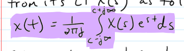
Inverse LT

c is a constant to ensure convergence of the integral; contour integral indicates that the LT indeed represents a CT signal as a sum of exponentally varying sinusoids

Partial Fraction Expansion (PFE) Approach

1. break LT X(s) fown into simpler components via PFE

2. find the inverse LT of the simpler components via table look-up

3. sum the inverse LTs to arrive at the inverse LT x(t)

only applicable when the LT is a rational function → a ratio of polynomials in s

LT Properties

linearity, time-shifting, frequency-shifting, time-differentiation, time-integration, time convolution, and LCCDEs

Linearity

x1(t) ←> X1(s) + x2(t) ←> X2(s) then ax1(t) + bx2(t) ←> aX1(s) + bX1(s)’ a and b are any constants (linear combination)

Time shifting

x(t) ←> X(s) then x(t-to) ←> e^(-sto) X(s) = e^(-(sigma + jw)to x(s)

x(t) is causal and can be viewed as x(t)u(t) to be more explicit

property is useful for determing the LT of signals w/ diff. time intervals

Frequency-shifting

x(t) ←> X(s) then x(t)e^(Sot) (exponential-varying sinusoid) ←> X(s-So)

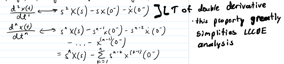
Time-differentiation

x(t) ←> X(s) then dx(t)/dt ←> xX(s) - x(0-)

Time Integration

x(t) ←> X(s) then the running integral (integral from 0- to t of x(T) dT ←> X(s)/s

Time Convolution

x1(t) ←> X1(s) + x2(t) ←> X2(t) then x1(t) * x2(t) ←> X1(s) X2(s)

if convolve 2 signals in time, multiply their LTs

Implication of Time convolution Property

flipping and sliding can be circumuated as follows

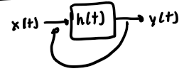
1. compute the LT of x(t) to get X(s) and the LT of h(t) to get H(s) (system fcn)

2. compute Y(s) = H(s) X(s) (multiplication)

3. take inverse LT of Y(s) to get y(t)

LCCDEs Revisited

time differentiation property of the LT along w/ the PFE approach for determing the inverse LT make LCCDE analysis easy

Total Response

can be decomposed into ZSR and ZIR; sum ZIR and ZSR to get original this;

ZSR and ZIR

forced response and natural response can be determined from these but not vice versa; they are general

H(s) - the system fcn for an LCCDE

P(s)/Q(s) = Y(s)/X(s); can be inverse transformed to arrive at the impulse response h(t) of an LCCDE

System Function for a CT LTI System

H(s) = Y(s)/X(s) = P(s)/Q(s) = Y{h(t)}; detrmines the complex scale factor applied by the system to inputs of the form e^(Sot) → y(t) = H(So)e^(Sot)

Q(s)

characteristic polynomial

P(s)

the “input” polynomial

What happens if P(s) and Q(s) have common factors?

roots of the numerator + denominator polynomials of H(s) are NOT the same as the input and characteristic polynomials

Poles

roots of the denominator polynomial; after common factors are canceled (if there is any)

Zeros

roots of the numerator polynomial; H(s) = 0

Pole-Zero Diagrams

indicate the location of the system poles and zeros in the s-plane; pole denoted w/ an X and a zero is denoted w/ an O

A causal system is?

1. BIBO stable if its poles are in the left-half s-plane (LHP)

2. unstable if poles in the RHP

3. marginally stable if there are no poles in the RHP but pole(s) on the jw-axis

ZERO LOCATIONS ARE NOT RELEVANT FOR STABILITY

Frequency Response

H(jw) as a fcn of w

Sinusoidal Input

x(t) e^st where sigma=0 so x(t)^jwot

system function: e^(sot)→[H(s)]→H(so)e^(sot)

output: y(t)=H(jwo)e^(jwot)=|H(jwo)|e^(j(wot + angleH(jwo)) only valid for BIBO stable systems

LTI systems do not alter what?

the frequency of sinusoid inputs

H(jw)

fcn of w reflects the filtering characteristics of the system

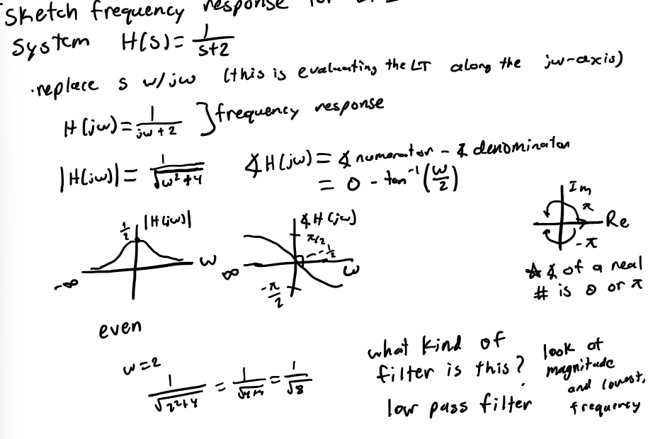
|H(jw)|

tells what teh frequencies are passed and surpressed by the system; vs w is the magnitude response

angle H(jw)

phase response

Sketching Frequency Response for LTI Steps

1. replace s w/ jw (evaluates the LT along the jw-axis)

2. find angle of H(jw) → numerator-denominator

3. sketch both

Sinusoidal Input Output Formula

y(t) = |H(jw)|*e^(j(wot + angle H(jwo))

onyl valid for BIBO stable systems

Response to Causal Sinusoidal Inputs

know H(s) = P(s)/Q(s) = P(s)/((s-lambda1)(s-lambda2)…(s-lambdan)) and Y(s) = H(s)*X(s) = P(s)/((s-lambda1)(s-lambda2)…(s-lambdan)(s-jwo))

apply PFE

Comments

acts of turning on an input at time 0 induces a natural response of the system even when the system is initially at rest; if x(t) = e^(jwot), at any finite time, the transient has long vanished leaving only the steady-state response so e^(jwot) → H(jwo)e^(jwot)

Bode Plots

the magnitude and phase responses sketched onto log scale plots; exploits asymptotic behaviors; simple way to plot the frequency response LTI systems on log scale

Bode Plot Steps

1. put it in “form” (factor out constants)

2. write magnitude and phase responses

3. take 20log of each

4. sketch each individual piece

5. add them up

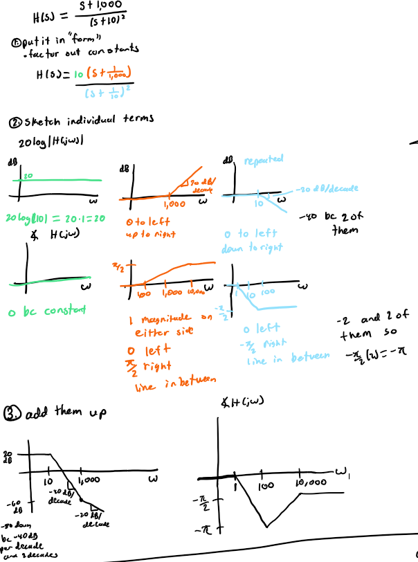
Constant - Individual Term

20log(#) for magnitude; angle is always 0 bc assume all parameters are positive

Pole or Zero at Origin - Individual Term

+ → is zero and - → pole; line has a slope of +- 20 dB/decade crossing the x-axis at w = 1 on log scale; angle is +- pi/2

Arbitrary Pole or Zero - Individual Term

gamma = ai = bi; 0 when w«gamma and +-20log(w)+-20log(gamma) when w»gamma (linw with slope +- 20 dB/decade crossing the x-axis at w=gamme on a log scale); angle = +- tan^-1(w/gamma) and is 0 when w«gamma and +-pi/2 when w»gamma

Feedback

the process of using the output of the system to continually alter its input; basis for many biological systems and other practical systems; LT techniques facilitate the analysis of these systems

Negative Feedback

system input is adjusted opposite to the direction to which the output is moving; biological systems specifically operate via this

Black’s Formula

overall system function = (forward path)/(1 - loop)