STAT1070: Statistics

Continuous variables

Numerical values measured as part of a whole and can take on any value e.g. percentages, fractions, times. Time and age are always continuous variables.

Discrete variables

Finite numbers that are counted not measured e.g. people (you can’t have half a person)

Nominal variables

Categorical variables that have no natural order. This also includes numerical data that acts as a symbol e.g. post codes or coded variables (1 = yes, 2 = no or outcomes)

Ordinal variables

Categorical variables with a natural order or scale but not with equal intervals e.g. grades.

Population

The entire group that the researcher is interested in and that is used to select the sample.

Sample

Selection/subset of data (ideally representative) from the population of interest

Paramters

Property of the population that you use the statistic to infer. μ (mean), X (observation), σ (SD), P (proportion) and N (size)

Statistics

Property of the sample that you use to infer parameters. x̄ (mean), n (size), x (observation), s (SD), p-hat (proportion).

Graph for ordinal data.

Bar charts (categories on x axis)

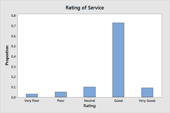
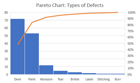
Graph for nominal data

Pareto chart (line = cumulative percentage) or bar chart for few categories

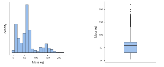
Graph for continuous data

Histogram or box plot

Graph for discrete data

bar chart (few outcomes) or histogram (many outcomes or the data is sparse)

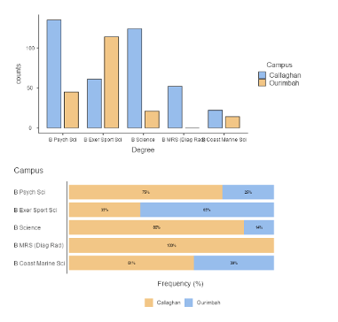
Graph for two categorical variables

Clustered bar chart (frequencies) or stacked bar chart (proportions) helps with seeing relative difference

P-value

The probability of obtaining a result equal to or more extreme than test statistic if the null hypothesis was true i.e. how likely the observed difference between groups is due to chance. Represents the chance of getting the test statistic or something more extreme, and the test statistic value is how close the data is to the null hypothesis.

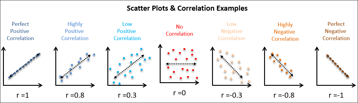
Correlation

A relationship between two or more things that is measured by the correlation coefficient (strength (0/1) and direction of relationship (-/+)) which indicates the extent to which changes in one variable are related to changes in another)

Coefficient of determination (R²)

Measure of proportion of variance in the dependent variable that can be explained by the independent variable in a regression model. Represents the goodness-of-fit of the regression model and ranges from 0 to 1 with higher = better fit.

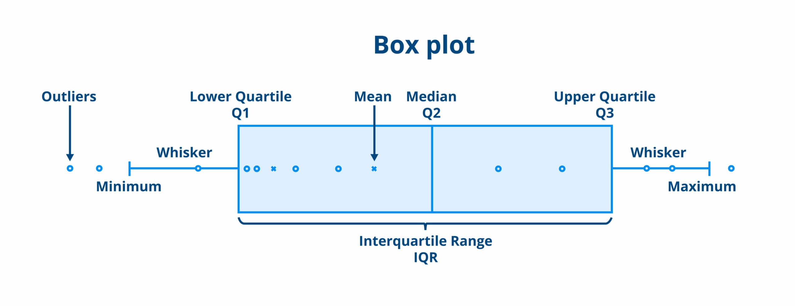
Inter Quartile Range (IQR)

Measures the spread of the middle half (50%) of your distribution excluding the outliers. Found by measuring the range between the first quartile (lower) and the third quartile (upper) (Q₃ - Q₁)

Large test Statistic

It is less likely that your data could have occurred under the null hypothesis

Mean (measure of central tendency)

The average by adding all the data points together and dividing by the number of data points

Median (measure of central tendency)

The middle number of data when sorted into ascending/descending. Divides the data into two equal halves with 50% of observations being above and 50% being below to median.

Non-parametric test

Statistical test that doesn't rely on specific assumptions about distribution of data. Used when data doesn't meet assumptions required for parametric tests. Based on ranks or ordering of data and suitable for analysing categorical or ordinal data.

Power (Beta)

Probability of correctly rejecting a false null hypothesis. Measures the ability of a statistical test/study to detect a true effect or relationship. Higher power = higher likelihood of detecting a true effect

Regression Slope (coefficient or beta coefficient)

Measure of change in dependent variable associated with a one-unit change in independent variable in a regression mode. Represents the slope of the regression line and the strength/direction of the relationship between variables

Rules of probability

Addition rule = P(A or B) = P(A) + P(B) - P(A and B); Conditional rule = P(A|B) = P(A and B)/P(B)

Standard deviation

A measure of dispersion/spread of numerical data that quantifies the average amount of deviation of each data point from the mean. Higher SD = greater variability

Type I error (a)

Null hypothesis is rejected even though it is true (incorrect rejection of a true null hypothesis). It represents probability of falsely concluding a relationship between variables when there is none.

Type II error (b)

Null hypothesis isn't rejected even though it is false (failure to reject a false null hypothesis). It represents the probability of failing to detect relationship between variables when there is one.

Z score

Quantifies distance between a data point and the mean of a data set to show you how many standard deviations the value is from the mean. Allows for standardisation.

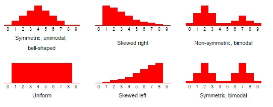
Shape

Symmetrical (normal distribution), positive (right) skewed, negative (left) skewed, or uniform. Helps identify appropriate measure of centre/spread: symmetrical = mean and SD, skewed = median and IQR (+ mean and SD). Distributions can also be unimodal = one peak/mode or bi/multi modal.

Spread

Measured through range, variance, SD, and IQR.

Variance

The spread between numbers in a data set. Determines how far each number is from the mean and other numbers in the set. Used to determine SD.

Observational Study

Researchers observe participants with no manipulation of variables to assess the relationship/behaviour in natural setting

Experimental study

Uses random allocation of participants to establish cause-and-effect relationships AND manipulates/controls variables and measures outcome

Longitudinal study (observational)

follows a group of participants over an extended period to examine changes/trends and help establish temporal precedence. Involves collecting data at multiple time points from the same participants

Cross sectional study (observational)

Where you collect data from participants at a single point in time which provides a snapshot of populations characteristics.

Cohort study (observational)

Group of people with common characteristic are followed over time to find how many reach a certain health outcome of interest. Examines the relationship between exposure to certain factors and the development of outcomes/disease

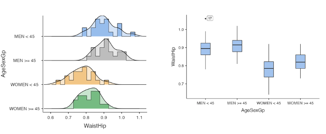
Graphs for continuous (y) and categorical (x) variables

Side-by-side box plots (centre/spread) or vertically aligned histograms (shape)

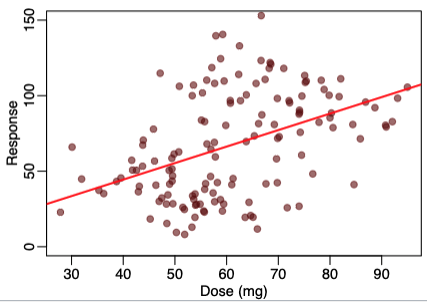
Graph for two continuous variables

Scatterplots

Describing scatterplot relationships

Consider strength (strong or weak), linear or non linear, and positive or negative. Non-linear relationships examples: exponential patterns or v shapes (can comment on strength but not direction)

Outliers

Observations that deviate from distribution pattern caused by natural variation or measurement error. You should always try and explain outliers to discount error.

1.5IQR rule

Suspected outliers are values at least 1.5 x IQR above Q3 or below Q1. Values below Q1 - 1.5IQR are low outliers (lower threshold) and values above Q3 + 1.5IQR are high outliers (upper threshold).

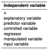
Independent (explanatory) variable

Manipulated/controlled and causes changes in the DV. It’s plotted on the x axis (horizontal)

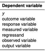
Dependent (response) variable

Measured and records the outcome. It is dependent on the IV and plotted on the y axis (vertical)

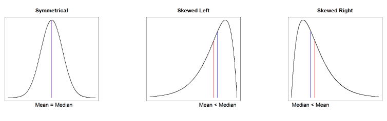
How does the shape of distribution change the relationship between mean and median and why?

Symmetrical: mean = median, skewed left: mean < median, and skewed right: mean > median. This is because the mean is affected by outliers i.e. when skewed left there are more low value outliers that decrease the mean but when skewed right there are more high value outliers that increase the mean.

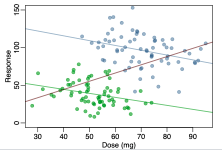
Graph for two continuous and one categorical variable

Scatterplot that has a key for the categorical data e.g. different colours or symbols for the different categorical levels.

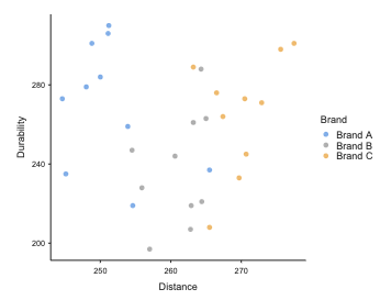
Table to describe one categorical variable.

Includes raw (counts) and relative (proportions) frequencies and is the table version of a bar chart.

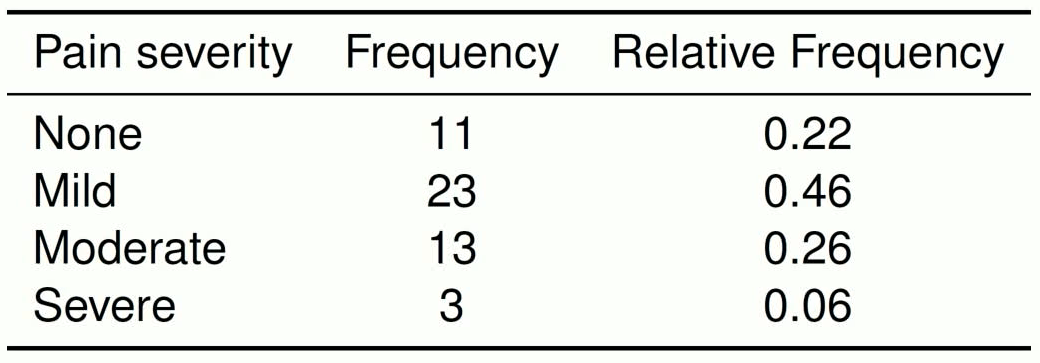
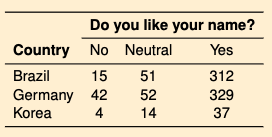
Table to describe two categorical variables

Contingency table/cross tabulation that combines two frequency tables to summarise the relationship between the two variables.

Bias

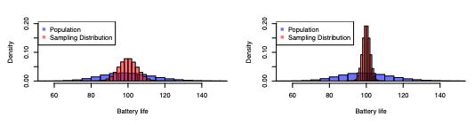
Related to the location of a statistic sampling distribution compared to the location of the true parameter value. If difference is 0 the sample is unbiased. To reduce the bias you use random sampling.

Precision

Related to the spread of sampling distribution i.e. less spread = more precise. You can improve precision by increasing the sample size.

Sampling error

The difference between statistic and parameter that is unavoidable but can be reduced in larger samples

Non-sampling error

Any error not caused by sampling size e.g. selection bias and measurement bias

Simpsons paradox

Description of a linear relationship when data is combined is positive however when split into groups it is negative (and vice versa)

3 R’s of study design

Randomisation, replication and reducing variation (blocking)

Simple random sampling (probability)

Researchers randomly select members of the population with each member having an equal probability of being selected.

Stratified sampling (probability)

Divide the population into subgroups and randomly sample from each subgroup. This can reduce bias and increase precision.

Cluster sampling (probability)

Split population into groups then randomly select groups and test the entire group e.g. schools. It has the potential of bias and there is limited choice for subgroup representation.

Sequential/systematic sampling (non-probability)

Systematic selection of a sample. Uses a sampling interval determined by population size/desired sample e.g. select every 10th

Convenience sampling (non-probability)

Sample readily available participants however it can cause highly biased data.

Snowball sampling (non-probability)

Sample by using one participant to find others e.g. “do you know anyone else who could participate in the study”

Line-intercept sampling (non-probability)

Line is chosen and any elements in that line form the sample e.g. flight patterns

Sensitivity

The probability of a test or measure to have a true positive result of the condition/disease = P(Positive test|Disease present)

Specificity

The probability of a test or measure to have a true negative result of the condition/disease = P(Negative test|No disease)

Probability notation

P(x) = probability of x event occurring which is always between 1 and 0

P(x^c) = probability of a complementary event occurring e.g. x not occurring

Mutually exclusive events

When two (or more) events can’t occur at the same time e.g. roll a 2 and 3 on one die roll.

Collectively exhaustive events

Set of events that encompasses all possible outcomes e.g. 1, 2, 3, 4, 5, and 6 for a die roll.

Marginal probability

The probability of a single event occurring = P(A)

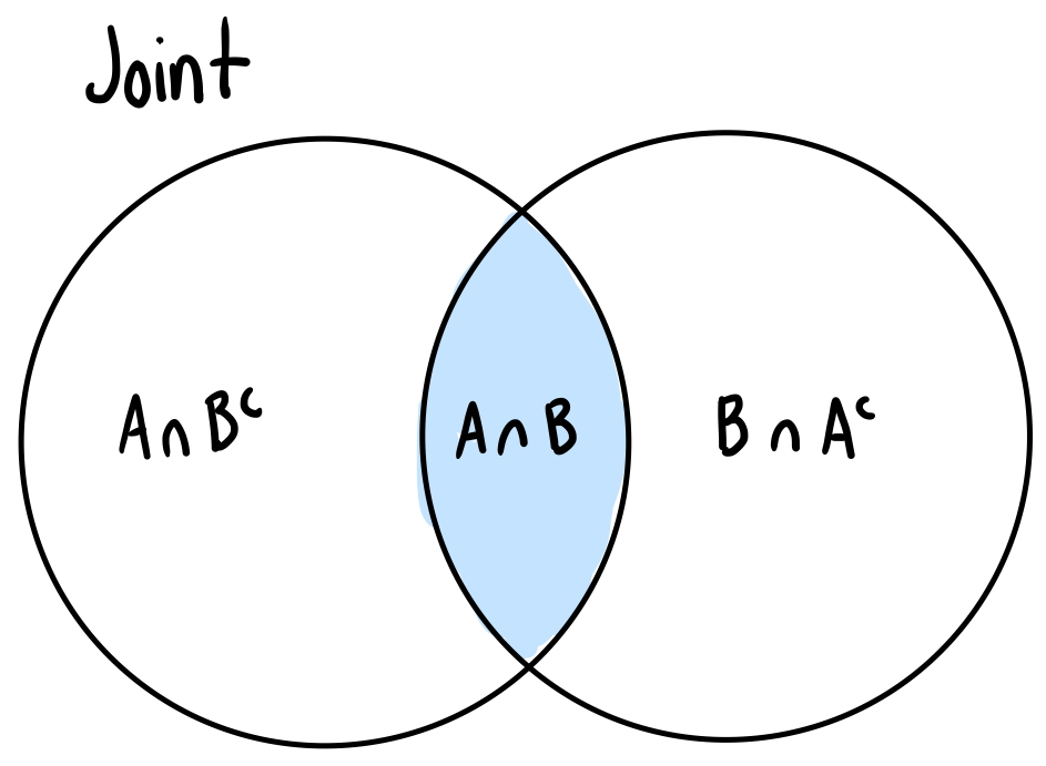
Joint probability

Probability of the intersection of two events = P(A ∩ B)

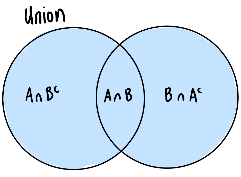
Union probability

The probability of A or B or both occurring = P(A ∪ B)

Conditional probability

The probability of two events where A is going to happen given B has already happening = P(A|B)

Probability rules

Union rule: P(A∪B) = P(A) + P(B)

Addition rule: P(A or B) = P(A) + P(B) - P(A and B)

Conditional rule: P(A|B) = P(A ∩ B) divided by P(B)

Joint (rearrangement of conditional rule): P(A∩B) = P(A|B) x P(B)

Independent events

Whether A event happens or not has no effect of P(B). Determined by either equation (you only need to test one):

P(A∩B) = P(A|B) x P(B)

P(A|B) = P(A)

P(B|A) = P(B)

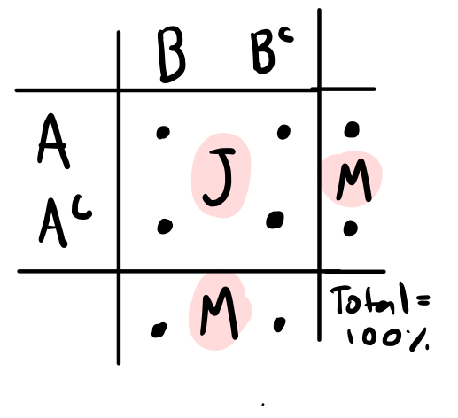
Contingency tables

Useful for joint and marginal probabilities

Venn diagrams

More useful for graphical representations than calculations.

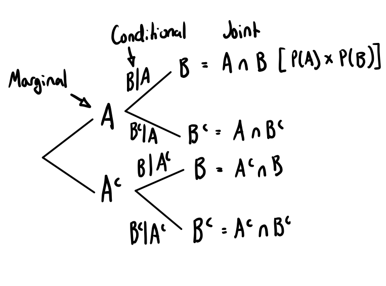
Tree diagrams

Useful for marginal and conditional probabilities

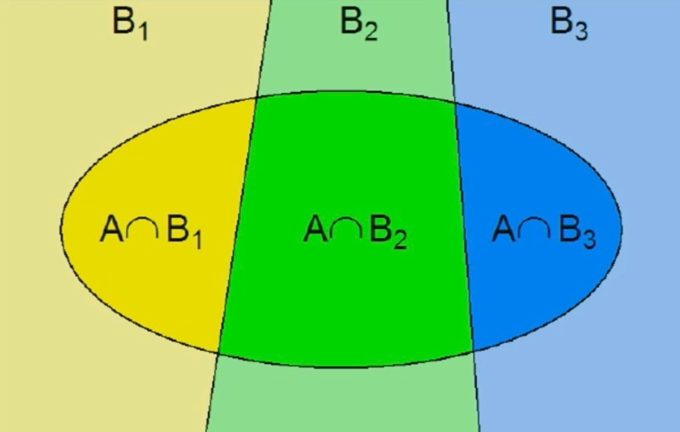
Partition

Set of mutually exclusive and collectively exhaustive events (e.g. states and the country)

Law of total probability

The total probability of an marginal event using the sum of conditional or joint events.

Joint: P(A) = P(A∩B₁) + P(A∩B₂) + etc..

Conditional: P(A) = P(A|B₁) x P(B₁) + P(A|B₂) x P(B₂)

Bayes rule

Used to invert conditional probabilities.

P(A|B) = P(B|A) x P(A) divided by P(B)

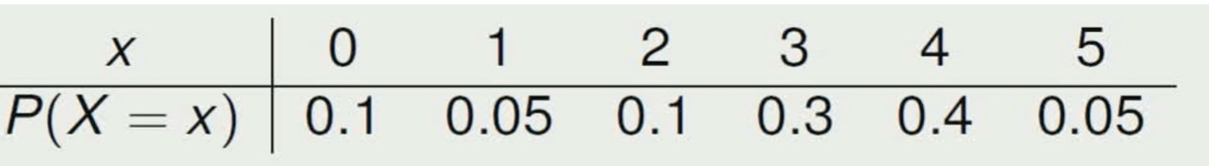
Probability distribution

Describes probabilities of experimental outcomes using data or models. Models provide a formula to define distribution of probabilities for numerical random variables.

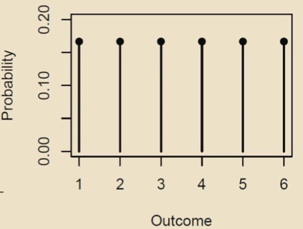
Discrete uniform probability distribution

All probabilities in sample space are evenly distributed across outcomes.

Function: P(X = x) = 1/n

Mean: n+1/2

Variance: (n+1) x (n-1)/12

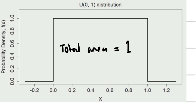
Continuous uniform probability distribution

Function: X ~ D (a,b) a (lower) and b (upper) = range.

Density function: f(x) = 1/b-a where a is less than or equal to x and b is greater than or equal to x AND f = height of density function

Higher value of density function means observing values in that region is more likely. The probability of a particular continuous outcome = 0

Population mean and standard deviation

Population mean = expected value E(X)

Population standard deviation = variance Var(X)

Random variables

Represented by X, they represent the result of chance outcome. The probability of a random variable = P(X = x)

Binomial variable criteria

Variable has fixed no. of trials, 2 possible outcomes (success or failure), constant probability of success, and trials are independent (e.g. random sample)

Binomial distribution

A discrete distribution represented by X ~ B (n, p) with n = no. of trials and p = probability of success

Binomial probability mass function

P(X = x) = (nCx) ⋅ p^x ⋅ (1-p)^n-x = probability of observing x successes out of n independent trials

nCx = binomial coefficient that counts the no. of ways to arrange x successes in n trials (often represented as a fraction w/o C)

p^x ⋅ (1-p)^n-x = probability of each sequences of x successes in n trials

Binomial distribution mean and variance

Mean = E(X) or μ = np

Variance = Var(X) or σ² = np(1-p)

Normal distributions

Most common continuous distribution that is completely characterised (and calculated) by mean. It must be symmetric and bell shaped and the measures of centre (mean, mode, median) must be equal.

Normal probability density function

Represented by X ~ N (μ, σ²) with μ = mean and σ² = variance or standard deviation squared.

Empirical rule

68% of values lie within ± 1 SD of mean

95% of values lie within ± 2 SD of mean

99.7% of values lie within ± 3 SD of mean

Standard normal distribution (z score)

Z ~ N (0,1) = standard normal distribution has mean of 0 and SD of 1. You can convert any random variable into a z-score using z = x - μ divided by σ.

Quantile

An observed value for a given probability statement. Can be applied to normal distributions in statstar.

Point estimation

Single value estimate of a parameter based on sample data e.g. mean μ with x̄

Interval estimate

Confidence intervals that estimate where the true population parameter lies between two values with a certain degree of confidence.

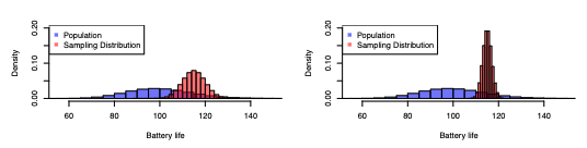
Central limit theorem

Can be applied to any numerical variable with finite population mean and sd which allows us to estimate μ and standard error with distribution of sample mean because we know the sample mean will be approximately normal even if population is skewed (allows for empirical rule). Assumptions:

• Population μ = sample mean x̄ (its a unbiased estimate)

• Standard error = σ / √n as we increase sample size the standard error decreases → more precise μ estimates

• Sample sizes >30 will be approximately normally distributed even if X isn’t

Hypothesis test steps

1. Null and alternative hypothesis = H₀: no effect/no relationship e.g. μ = μ H_A: difference/relationship μ ≠ μ

2. Test statistic =. summarise difference between means/values

3. Determine null distribution = distribution of test statistic assuming H₀ is true

4. P-value = probability of getting the test statistic or more extreme

5. Decision = p < significance level (e.g. 0.05) → reject H₀ or vice versa

6. Conclusions = reject or fail to reject null hypothesis due to evidence (p-value)

*check assumptions: differ depending on test

Confidence intervals

Formula = sample mean ± multiplier x margin of error. Multiplier changes based on confidence. Can be used as an alternate to hypothesis testing e.g. whether or not the μ is in the confidence interval.

Z-test

Uses z scores and the empirical rule to make inferences on p-values and confidence internals. Follows same hypothesis test except the test-statistic is a z-score,

Two-tailed vs one-tailed hypothesis test

One tailed = checks difference in one direction e.g. greater than or less than

Two tailed = checks difference in both directions e.g. greater than and less than

Margin of error

z score x σ / √n

As you increase sample size the ME gets smaller, width of CI represents 2 x ME meaning as you increase confidence the ME and CI increases.

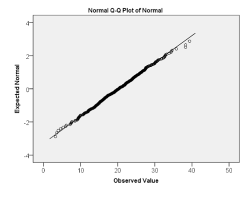
Q-Q normal quantile plot

A method of assessing normality by plotting observed data and theoretical quantiles from a normal distribution. If data is normally distributed then the points should approximate a straight line. If there is a clear curve or S shape then that indicates it may not be normally distributed.