Biostatistics 281 Chapters 1-6 MIDTERM Study Guide

Statistics

• A way of learning from data 

• Concerned with all elements of study design, data collection, and analysis of numerical data

• Requires judgement

Biostatistics

Statistics applied to biological and health problems

Data Judges

Judge and confirm clue

Use statistical inference

Data Detectives

Uncover patterns and clues

Use exploratory data analysis and descriptive statistics

Goals of Biostatistics

Improvement of the intellectual content of data

Organization of data into understandable forms

Reliance of tests of experience as a standard of validity

Data Collection Form

• Observation:

  • Unit upon which measurements are made, can be individual or aggregate

•  Variable:

  • The generic thing we measure 

  • Examples: Age, HIV status

• Value: 

  • A realized measurement

  •  Examples: “27”, “positive”

Data Table

Each row corresponds to an observation

Each column contains information on a variable

Each cell in the table contains a value

Data Dictionary

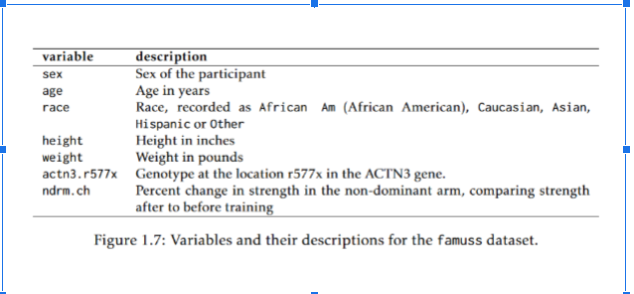
Types of Measurements

The assigning of numbers and codes according to prior-set rules.

Categorical - Nominal

No implied order of categories

E.g., Race, sex, colors

Categorical - Ordinal

Categories can be placed in some order

E.g., Likert Scales (Strongly agree, agree, no opinion, disagree, strongly disagree)

Numerical - Discrete

Counts or whole numbers

E.g., number of patients, number of children in a family.

Numerical - Continuous

Can take on any value within a range

E.g., height, weight, temperature

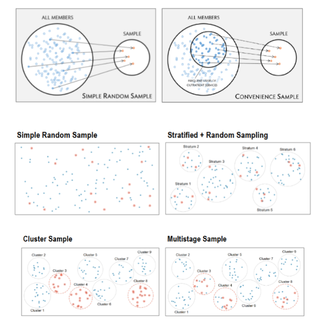
Population vs. Sample

Saves time

Saves money

Allows resources to be devoted to greater scope and accuracy

Sampling Methods

Precision - Imprecision

Inability to be replicated

Precision - Bias

Tendency to overestimate or underestimate the true value of an object.

Many different types of biases exist, below are a few examples

• Selection Bias

• Detection Bias

• Omitted Variable Bias

• Attrition Bias

• Non-Response Bias

• Response Bias

Symmetry

Degree to which shape reflects a mirror image of itself around its center

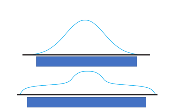
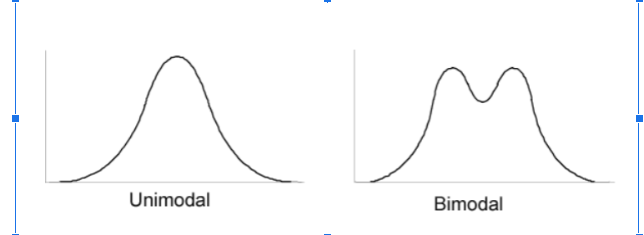
Modality

Number of peaks

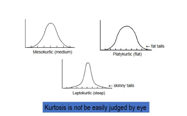
Kurtosis

Steepness of the mound (width of tails)

Departures

Outliers

Skew Example

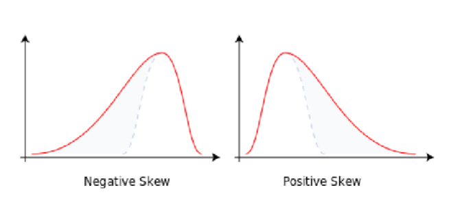
Two examples of chart

Arithmetic Average (Mean)

Gravitational Center

Median

Middle Value

EXAMPLE - order the data from lowest to highest

• 5 11 21 24 27 28 30 42 50 52

• The median has a depth of (n + 1) ÷ 2 on the ordered array

• When n is even, average the points adjacent to this depth 

• For illustrative data: n = 10, median’s depth = (10+1) ÷ 2 = 5.5 

• The median falls between 27 and 28

What is included in the spread?

• Range

• Inter-Quartile Range

• Standard Deviation

• Variance

Range

• Minimum to maximum

• The easiest but not the best way to describe spread (e.g., standard deviation, etc.) 

• The range is “from 5 to 52” 

  • 5 11 21 24 27 28 30 42 50 52

Frequency Table

• Frequency

  • Count

• Relative Frequency

  • Proportion or %

• Cumulative Frequency

  • % less than or equal to level

• When data are sparse, group data into class intervals

• Create 4 to 12 class intervals

• Classes can be uniform or non-uniform (TRY TO KEEP IT UNIFORM!)

• End point convention: e.g., first class interval of 0 to 10 will include 0 but exclude 10 (0 to 9.99)

• Talley frequencies

• Calculate relative frequency

• Calculate cumulative frequency

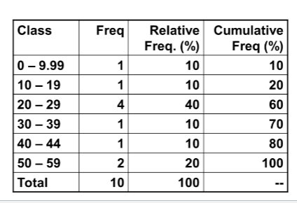
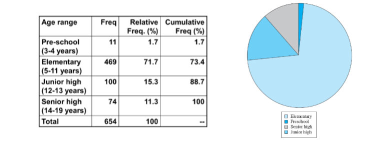
Frequency Table Example #1

• Uniform class intervals table (width 10) for data:

  • 05, 11, 21, 24, 27, 28, 30, 42, 50, 52

• Create a Frequency Table

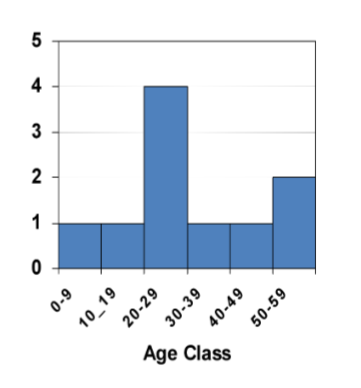
Histogram

• A histogram is a frequency chart for a quantitative measurement

• Notice how the bars touch

Bar Chart

A bar chart with non-touching bars is reserved for categorical measurements

Pie Chart

Summary statistics

• Central Location 

  • Mean 

  • Median

  • Mode

• Spread

  • Range and interquartile range (IQR)

  • Variance and standard deviation

• Shape

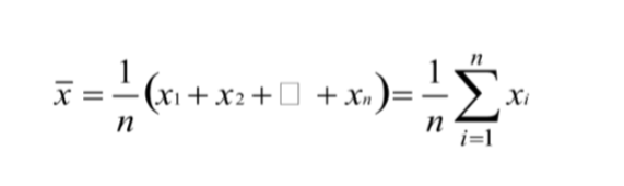
Notation

• n = sample size 

• X = the variable (e.g., ages of subjects) 

• xi = the value of individual i for variable X

• Σ = sum all values (capital sigma) 

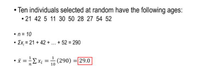
  • Example (ages of participants): 

    • 21 42 5 11 30 50 28 27 54 52 

      • n = 10

      • X = AGE variable 

      • x1 = 21, x2 = 42, ..., x10 = 52 

      • Σxi = x1 + x2 + ... + x10 = 21 + 42 + ... + 52 = 290

Central Location (Sample Mean)

• “Arithmetic Average”

• Traditional Measure of Central Location

• Sum the values and divide by n

• X refers to the sample mean

Central Location (Sample Mean) EXAMPLE

The mean is the balancing point of a distribution

gravitational center

• Susceptible to skews

• Can be used to predict…

  • Randomly values from sample

  • Random values from population

  • Population mean

Central Location (Median)

• Order the data from lowest to highest 

  • 5 11 21 24 27 28 30 42 50 52 

• The median has a depth of (n + 1) ÷ 2 on the ordered array 

• When n is even, average the points adjacent to this depth 

• For illustrative data: n = 10, median’s depth = (10+1) ÷ 2 = 5.5 

• The median falls between 27 and 28. Median = 27.5

• The median is more resistant to skews and outliers than the mean; it is more robust. 

• It is less impacted by skewness and outliers. 

• 1362 1439 1460 1614 1666 1792 1867 

  • Mean = 1636 

  • Median = 1614 

• 1362 1439 1460 1614 1666 1792 9867 

  • Mean = 2743

  • Median = 1614

Central Location (Mode)

• The mode is the most commonly encountered value in the dataset

• This data set has a mode of 7

  • {4, 7, 7, 7, 8, 8, 9} 

• This data set has no mode 

  • {4, 6, 7, 8} 

• The mode is useful only in large data sets with repeating values

Effect of a Skew on the Mean, Median, and Mode:

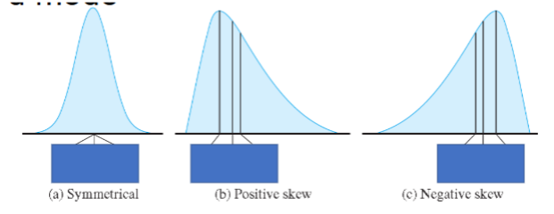
Note how the mean gets pulled toward the longer tail more than the median

• mean = median → symmetrical distribution 

• mean > median → positive skew 

• mean < median → negative skew

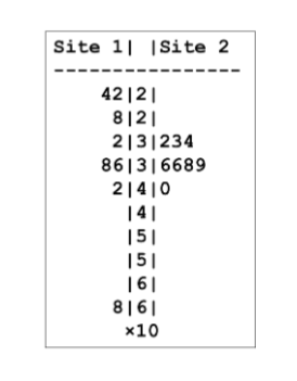
Spread

• Two distributions can be quite different yet can have the same mean. 

• This data compares particulate matter in air samples (μg/m3) at two sites. 

• Both sites have a mean of 36, but Site 1 exhibits much greater variability. 

• We would miss the high pollution days if we relied solely on the mean.

Spread (Range)

• Range 

• Maximum – minimum 

• Site 1 range is from 22 to 68 (range of 46) 

• Site 2 range is from 32 to 40 (range of 8) 

• Beware: the sample range will tend to underestimate the population range. 

• Always supplement the range with at least one addition measure of spread

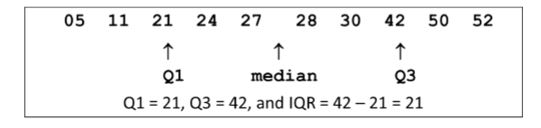
Spread (Quartiles)

• Quartile 1 (Q1): 

  • Cuts off bottom quarter of data 

  • Median of the lower half of the data set 

• Quartile 3 (Q3) 

  • Cuts off top quarter of data 

  • Median of the upper half of the data set 

• Interquartile Range (IQR) 

  • Q3 – Q1 

  • Covers the middle 50% of the distribution

Spread (Quartiles) - Example

• You are given a SRS of metabolic rates (cal/day), n = 7 

• 1362 1439 1460 1614 1666 1792 1867 

• When n is odd, include the median in both halves of the data set. 

• Bottom half: 1362 1439 1460 1614 

  • Median = 1449.5 (Q1) 

• Top half: 1614 1666 1792 1867 

  • Median = 1729 (Q3)

Five Point Summary

• Q0 (the minimum) 

• Q1 (25th percentile) 

• Q2 (median) 

• Q3 (75th percentile) 

• Q4 (the maximum)

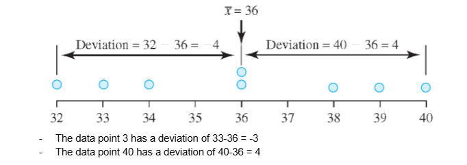
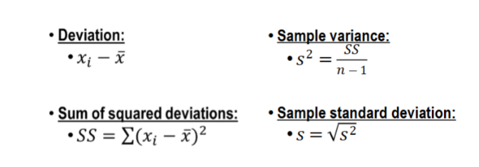
Standard Deviation

• Most common descriptive measures of spread 

• Based on deviations around the mean

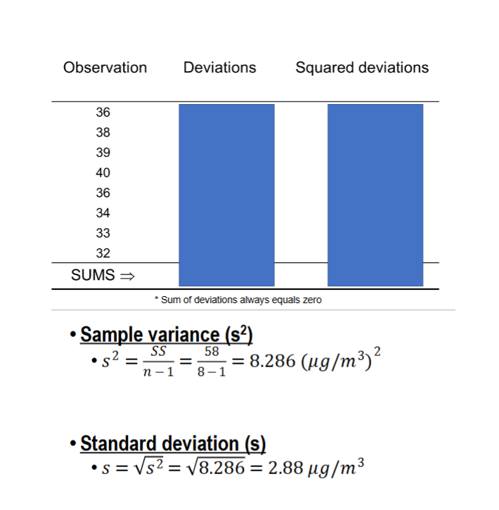
Standard Deviation EXAMPLE

This data set has a mean of 36.

FORMULAS

Example of using the formulas

Sample -> Population

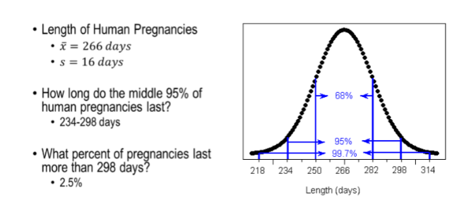
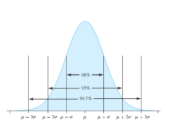
68-95-99.7 Rule

68-95-99.7 RULE (Example)

Chebyshev’s Rule

• ALL Distributions 

• Chebychev’s rule says that at least 75% of the values will fall in the range μ ± 2σ.

• Example: 

  • A distribution with μ = 30 and σ = 10 has at least 75% of the values in the range 30 ± (2)(10) = 10 to 50

Surveys

• Describe population characteristics 

• Example 

  • A study of the prevalence of hypertension in a population

Comparative Studies

• Determine relationships between variables 

• Example 

  • A study to address whether weight gain causes hypertension

Outline of Studies

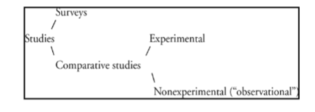
Comparative Studies

• Comparative designs study the relationship between an explanatory variable and response variable.

• Example: 

  • The first test you decide not to study and you get a C+. 

  • The second test you decide to study and get an A.

•  Explanatory

  • What you do to cause change. 

• Response

  • What you’re hoping to change.

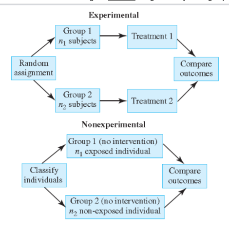
Comparative Studies - Experimental

Investigators assign the subjects to groups

Comparative Studies - Observational

Investigator does not assign the subjects to groups

Comparative Study Comparison

• In the experimental design, the investigators controlled who was and who was not exposed.

• In the non-experimental design, the study subjects (or their physicians) decided on whether or not subjects were exposed

Experimental Principles

• Controlled comparison

• randomized 

• replication

Controlled Trial

• Control Group = Non-exposed. 

• You can’t know how a treatment causes change without comparing it to someone who didn’t take the treatment. 

• You won’t know if studying before an exam helps without first not studying for it.

• You cannot judge effects of a treatment without a control group because: 

  • Many factors contribute to a response 

  • Conditions change on their own over time 

  • The placebo effect and other passive intervention effects are operative

Randomization

• Refers to randomly putting people into treatment groups. 

• Balances lurking variables among treatments groups, mitigating their potentially confounding effects

Replication

The results of a study conducted on a larger number of cases are generally more reliable than smaller studies

Ethics Outline

• Informed Consent

• Beneficence

• Equipoise

• Institutional Review Board

• Additional Ethical Principles

Informed Consent

Biostatisticians should obtain informed consent from research participants before collecting data. Informed consent involves providing participants with information about the study, including its purpose, procedures, risks, and benefits, and obtaining their voluntary agreement to participate.

Beneficence

Biostatisticians should maximize benefits and minimize harms to research participants and society. This principle involves ensuring that research is conducted in a way that promotes the well-being of participants and society.

Equipoise

Biostatisticians should ensure that the research question is scientifically valid and that the study design is appropriate to answer the question. This principle involves ensuring that the study is designed in a way that minimizes bias and confounding.

Institutional Review Board

Biostatisticians should work with IRBs to ensure that research is conducted in an ethical manner. IRBs are responsible for reviewing research proposals to ensure that they meet ethical standards and that the rights and welfare of research participants are protected.

Additional Ethical Principles

• Integrity of data and methods 

• Responsibilities to stakeholders 

• Responsibilities to research subjects, data subjects, or those directly affected by statistical practices

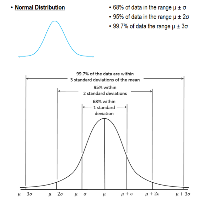
Normal Distributions

• Continuous random variables are described with smooth probability density functions (pdfs)

• Normal pdfs are recognized by their familiar bell-shape

• Example: Age distribution of a pediatric population

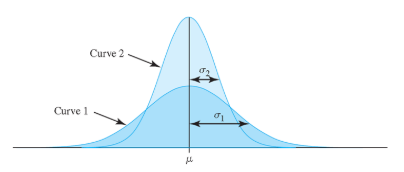
Parameters μ and σ

• Normal pdfs are a family of distributions

• Family members identified by parameters μ (mean)and σ (standard deviation)

μ controls location

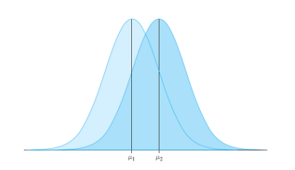
σ controls spread

68-95-99.7 Rule

Normal Distribution

• 68% of data in the range μ ± σ

• 95% of data in the range μ ± 2σ

• 99.7% of data the range μ ± 3σ

Reexpression of Non-Normal Variables

• Many variables are not Normal

• We can re-express non-Normal variables with a mathematical transformation to make them more Normal

• Example of mathematical transforms include logarithms, exponents, square roots, and so on.

Logarithms

• Logarithms are exponents of their base

• There are two main logarithmic bases

• common log₁₀

(base 10)

• natural ln

(base e)

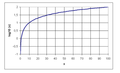
Landmarks

• log₁₀(1) = 0

(because 10⁰ = 1)

• log₁₀(10) = 1

(because 10¹ = 10)

Statistical inference

The act of generalizing from a sample to a population with calculated degree of certainty

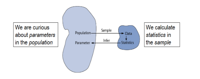
Population

• Represents everyone

• Mean → μ

• Standard Deviation → σ

Sample

• A subset of the population

• Mean → x ̅ (x-bar)

• Standard Deviation → s

Sampling Behavior of A Mean

• How precisely does a given sample mean reflect the underlying population mean?

• To answer this question, we must establish the sampling distribution of x-bar

• The sampling distribution of x ̅ is the hypothetical distribution of means from all possible samples of size n taken from the same population

Finding 1 (central limit theorem)

The sampling distribution of x-bar tends toward Normality even when the population distribution is not Normal. This effect is strong in large samples.

Finding 2 (unbiasedness)

The expected value of x-bar is μ

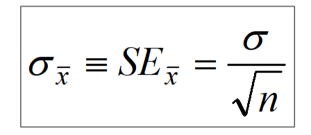
Finding 3 (square root law)

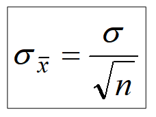
Standard Deviation (Error) of the Mean

• The standard deviation of the sampling distribution of the mean has a special name: it is called the “standard error of the mean” (SE)

• The square root law says the SE is inversely proportional to the square root of the sample size:

• What do you think would happen if we increase our sample size?

• Our SE or standard error of the mean would go down!

• As, ↑n → ↓σ

Law of Large Numbers

• As a sample gets larger and larger, the sample mean tends to get closer and closer to the μ

• This tendency is known as the Law of Large Numbers

Statistical Inference

Generalizing from a sample to a population with calculated degree of certainty

Two forms of statistical inference

• Hypothesis testing

• Estimation

Introduction to Hypothesis Testing:

• Hypothesis testing is also called significance testing

• The objective of hypothesis testing is to test claims about parameters

• For example, does a clinical study of a new cholesterol-lowering drug provide robust evidence of a beneficial effect in patients at risk for heart disease.

• A drug is considered to have a beneficial effect on a population of patients if the population average effect is large enough to be clinically important. It is also necessary to evaluate the strength of the evidence that a drug is effective; in other words, is the observed effect larger than would be expected from chance variation alone?

• A method for calculating the probability of making a specific observation under a working hypothesis, called the null hypothesis.

• By assuming that the data come from a distribution specified by the null hypothesis, it is possible to calculate the likelihood of observing a value.

• If the chances of such an extreme observation are small, there is enough evidence to reject the null hypothesis in favor of an alternative hypothesis.

Hypothesis Testing Steps

1. Formulating null and alternative hypotheses

2. Specifying a significance level (α)

3. Calculating the test statistic

4. Calculating the p-value

5. Drawing a conclusion

Null and Alternative Hypothesis

• The null hypothesis (H₀) often represents either a skeptical perspective or a claim to be tested.

• The alternative hypothesis (H_A) is an alternative claim and is often represented by a range of possible parameter values.

The logic behind rejecting or failing to reject the null hypothesis is similar to the principle of presumption of innocence in many legal systems. In the United States, a defendant is assumed innocent until proven guilty; a verdict of guilty is only returned if it has been established beyond a reasonable doubt that the defendant is not innocent. In the formal approach to hypothesis testing, the null hypothesis (H0) is not rejected unless the evidence contradicting it is so strong that the only reasonable conclusion is to reject H0 in favor of HA.

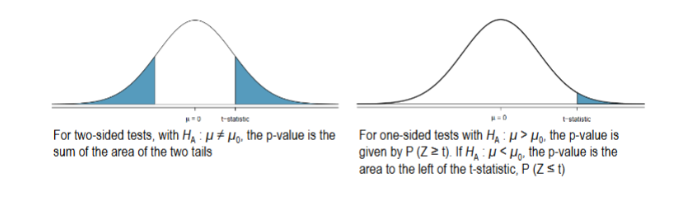
two-sided alternative.

The alternative hypothesis H_A : μ ≠ 0 is called a two-sided alternative.

Specifying a Significance Level (a)

• It is important to specify how rare or unlikely an event must be in order to represent sufficient evidence against the null hypothesis. This should be done during the design phase of a study, to prevent any bias that could result from defining ’rare’ only after analyzing the results.

• When testing a statistical hypothesis, an investigator specifies a significance level, α, that defines a ’rare’ event. Typically, α is chosen to be 0.05, though it may be larger or smaller, depending on context

Calculating the Test Statistic

• The test statistic quantifies the number of standard deviations between the sample mean x ̅ and the population mean μ.

• The perfect Normal distribution has a mean of 0 (μ = 0) and a standard deviation of 1 (σ = 1).

• If your data’s distribution does not match these parameters exactly, then you need to standardize to make it fit. Different standardization formulas exist depending on the specific statistical analysis that is being conducting.

• For example, a one sample t-test, the following formula would be used:

t=(x ̅-μ_0)/(s∕√n)

• s represents the sample standard deviation and n represents the number of observations in the sample.

Calculating the P-Value

• The p-value is the probability of observing a sample mean as or more extreme than the observed value, under the assumption that the null hypothesis is true.

• The p-value can either be calculated from software or from the normal probability tables. For the weight-difference example, the p-value is vanishingly small:

Drawing a Conclusion

• To reach a conclusion about the null hypothesis, directly compare p and α. Note that for a conclusion to be informative, it must be presented in the context of the original question; it is not useful to only state whether or not H₀ is rejected.

• If p > α, the observed sample mean is not extreme enough to warrant rejecting H₀; more formally stated, there is insufficient evidence to reject H₀.

• A high p-value suggests that the difference between the observed sample mean and μ₀ can reasonably be attributed to random chance.

• If p ≤ α, there is sufficient evidence to reject H₀ and accept H_A.

• Thus, the data support the conclusion that on average, the difference between actual and desired weight is not 0 and is positive; people generally seem to feel they are overweight.