Understanding One-Way ANOVA and Statistical Concepts

One-way ANOVA

One-way ANOVA (Analysis of Variance) is used to compare means across three or more groups based on one independent variable. It assesses whether at least one group mean significantly differs from the others.

Dependent variable

The dependent variable should be continuous (interval or ratio scale).

Independent variable

The independent variable should be categorical with 3 or more levels.

Assumptions of ANOVA

Assumptions include normality within groups, homogeneity of variances, and independence of observations.

Real-World Example of One-way ANOVA

A teacher compares the test scores (dependent variable) of three different teaching methods (independent variable with 3 levels: traditional, online, and hybrid). One-way ANOVA tests if the average scores differ across these methods.

ANOVA

Compares means across more than two groups simultaneously to avoid Type I errors (false positives).

Multiple t-tests

When you conduct multiple pairwise t-tests between group means, you increase the likelihood of committing a Type I error.

Real-World Example of Multiple t-tests

If you used multiple t-tests to compare test scores between each pair of teaching methods, you would inflate the error rate. ANOVA provides a more reliable overall comparison.

Post-hoc tests

After finding a significant result in ANOVA, post-hoc tests (like Tukey's HSD) are used to determine which specific groups differ from each other.

Interpretation of SPSS Output

SPSS will show the results of the ANOVA and any post-hoc tests. The p-values from post-hoc tests tell you which pairs of groups have significant differences.

Real-World Example of Post-hoc tests

After finding a significant difference in test scores between teaching methods, a post-hoc test (e.g., Tukey's) will reveal whether, for example, traditional vs. hybrid teaching methods differ significantly in scores.

One-Way ANOVA vs. Two-Way ANOVA

One-Way ANOVA involves one independent variable with 3 or more levels, while Two-Way ANOVA involves two independent variables, potentially allowing the study of both main effects and interaction effects between the two variables.

Real-World Example of Two-Way ANOVA

A study on test scores (dependent variable) that examines both teaching method (traditional, online, hybrid) and student gender (male, female) could use a two-way ANOVA.

Main Effect

The individual effect of each independent variable on the dependent variable.

Interaction Effect

The combined effect of two or more independent variables on the dependent variable.

Real-World Example of Main Effects vs. Interaction Effect

In a two-way ANOVA studying test scores by teaching method and gender, the main effect of teaching method tells you how different methods impact scores overall. The interaction effect tells you whether the impact of teaching method depends on gender.

Spreading Interaction

As one factor increases, the other has a consistent effect. The lines are not parallel but spread apart.

Crossover Interaction

The effect of one factor reverses direction at different levels of the other factor. Lines cross each other.

Spreading Interaction

A type of interaction where higher dosage always improves health, but more in the evening.

Crossover Interaction

A type of interaction where higher dosage helps in the morning but harms in the evening.

Pearson's r Correlation Coefficient

A measure of the strength and direction of the linear relationship between two continuous variables.

Direction of Correlation

Can be positive (both variables increase together) or negative (one increases while the other decreases).

Strength of Correlation

Ranges from -1 (perfect negative) to 1 (perfect positive), with values closer to 0 indicating a weak relationship.

Form of Correlation

Assumes a linear relationship.

Correlation Example

A study finds a correlation of 0.80 between hours studied and test scores, indicating a strong positive linear relationship.

Data Requirements for Pearson's r

Both variables must be continuous (interval or ratio scale), the relationship should be linear, and assumes normality of data for both variables.

Positive Correlation

As one variable increases, the other increases (e.g., more hours of sleep, better performance on exams).

Negative Correlation

As one variable increases, the other decreases (e.g., more hours of TV watched, lower test scores).

Correlation

Measures the strength and direction of the relationship between two variables.

Regression

Predicts the value of one variable based on the value of another.

Regression Example

Correlation tells you how strongly hours studied and test scores are related, while regression would allow you to predict a student's score based on the number of hours they studied.

Slope (b)

Represents the change in the dependent variable for each unit change in the independent variable.

Intercept (a)

The value of the dependent variable when the independent variable is zero.

Line of Best Fit Equation

The regression line is expressed as Y=a+bX, where Y is the predicted value of the dependent variable, a is the y-intercept, and b is the slope.

Interpreting Regression Equation

For every unit increase in X (independent variable), the dependent variable Y is expected to change by the amount of the slope (b).

Using Regression Equation

Plug in the value of X into the regression equation to compute the predicted value of Y.

Data Requirements for Chi-Square

Goodness of Fit: One categorical variable with a single sample, comparing observed frequencies to expected frequencies; Test of Independence: Two categorical variables, testing if they are independent or associated.

Goodness of Fit Test

Tests if the observed frequencies of a single categorical variable match expected frequencies.

Test of Independence

Tests if two categorical variables are independent or related.

Descriptive Statistics

Summarizes data (e.g., mean, median, standard deviation).

Inferential Statistics

Makes predictions or generalizations based on a sample (e.g., hypothesis testing, confidence intervals).

Measures of Central Tendency

Mean, median, mode.

Measures of Dispersion

Range, variance, standard deviation.

Hypothesis Testing

t-tests, ANOVA, chi-square tests.

Confidence Intervals

Estimating population parameters based on sample data.

Purpose of Hypothesis Testing

To determine whether there is enough evidence in a sample to infer that a particular condition holds true in the population.

p < Alpha Significance Level

If p<α (usually 0.05), it indicates strong evidence against the null hypothesis, leading to the rejection of the null hypothesis.

Null Hypothesis (H₀)

The assumption that there is no effect or relationship.

Alternative Hypothesis (H₁)

The assumption that there is an effect or relationship.

Directional Hypothesis

Specifies the direction of the effect (e.g., one group is greater than another).

Non-Directional Hypothesis

Does not specify direction (e.g., groups are different but no direction specified).

Repeated-Measures Design

Same participants are tested under different conditions (e.g., pre-test/post-test).

Independent Measures Design

Different participants are tested under each condition (e.g., comparing different groups).

Statistical Significance

The result is unlikely due to chance (based on p-value).

Practical Significance

The result has real-world importance, even if it is statistically significant.

Independent Variable (IV)

The variable manipulated to observe its effect on the dependent variable.

Dependent Variable (DV)

The outcome or response that is measured.

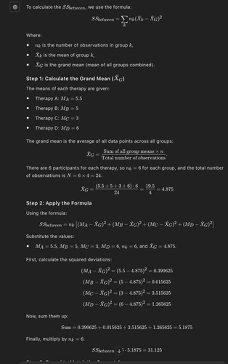
SSbetween

The average squared differences of the group means from the grand mean.

Post Hoc Test

A post hoc test is used after a significant ANOVA result to identify which specific group means differ significantly while controlling for Type I error.

SSwithin

The average squared differences of the individual scores from the group mean.

Two-Way ANOVA

2 main effects, 1 interaction.

Regression Form

The shape that the best line of fit takes through the individual values.

Regression Strength

The consistency at which individual values tend to cluster around a trend.

Regression Direction

The trend in which individual values tend change which can be the same or the opposite.

Sum of Products (SP)

Positive or negative.

Sum of Squares (SS)

Always positive.

Pearson r Correlations

Assess linear relationships between two quantitative variables.

Benefits of Scatterplot

Shows relationship is linear, defines outliers.

Simple Linear Regression

Tests the model of a relationship between two quantitative variables.

Regression Equation Interpretation

Y will be 2.42 when X is 0 and will decrease by .77 for each one unit increase in X.

Multiple Regression

Models the relationship between multiple continuous variables and a single continuous outcome variable.