3. Descriptive Statistics

Define the keyword “Entire Set / Population”

The “entire set” or the “population” is the set of all possible observations

Define the keyword “Sample”

A sample is a set of observations, drawn from the population/entire set.

Example: Roling the dice 5 times can e.g. result in: 2, 5, 2, 1, 3

Define the keyword “Number of Samples”

Number of observations (N = 5 in the example above → Roling the dice 5 times can e.g. result in: 2, 5, 2, 1, 3)

Define the keyword “Estimate”

Every statistical parameter derived from a sample is only an estimate. Only parameters taken from the entire set/population are considered to be the “truth” or the “true value”.

Define the keyword “Notation”

A statistical estimate (taken from the sample) is denoted with a “^” on top of the statistical parameter of the entire set / population. If μ is average of the population → \overline{\mu} is average of the sample.

Example: For roling the dice μ = 3,5. With the sample above “2, 5, 2, 1, 3” → \overline{\mu} = 2,6 .

\overline{\mu}

For roling the dice hundreds and thousands of times \overline{\mu} would converge towards μ, i.e.

\overline{\mu} →(N→ \infty ) μ

Define the keyword “Convergence”

As N becomes larger, every statistical estimate converges towards that of the entire set/population. I.e. N must be sufficiently large to be “representative”

Define the keyword “Real values”

In engineering we mostly deal with real valued physical quantities

Example: Total pressure of 12,3456 bar, i.e. theoretically and in general the set of all possible values is infinite. A limited precision during measurements will “discretize” real valued quantities

Why do we need statistics ? Whats the main challenge in engineering design and modelling and what is the solution for that problem/challenge?

Challenge = “The result parameters of a model/process scatter (are uncertain), because of the uncontrollable (scattering/uncertain) input parameters.”

• Getting rid of uncontrollable input parameters is neither possible nor financially viable. Example: Eliminating manufacturing tolerances would require “infinitely” accurate manufacturing machines → not possible!

Question: How can we accept we cannot change uncontrollable parameters and modify controllable input parameters to design an optimal and reliable product

Solution: Quantify the Scatter , i.e. the Statistics of the Results

Define “Statistical Parameters” and “Distribution”

Statistical Parameters: Parameters characterizing the shape of the scatter in terms of values for location, width, symmetry etc

Distribution: Characterizing and understanding scatter in terms of shape and probabilities

What paramter characterizes the shape of the scatter in “First statistical moment”

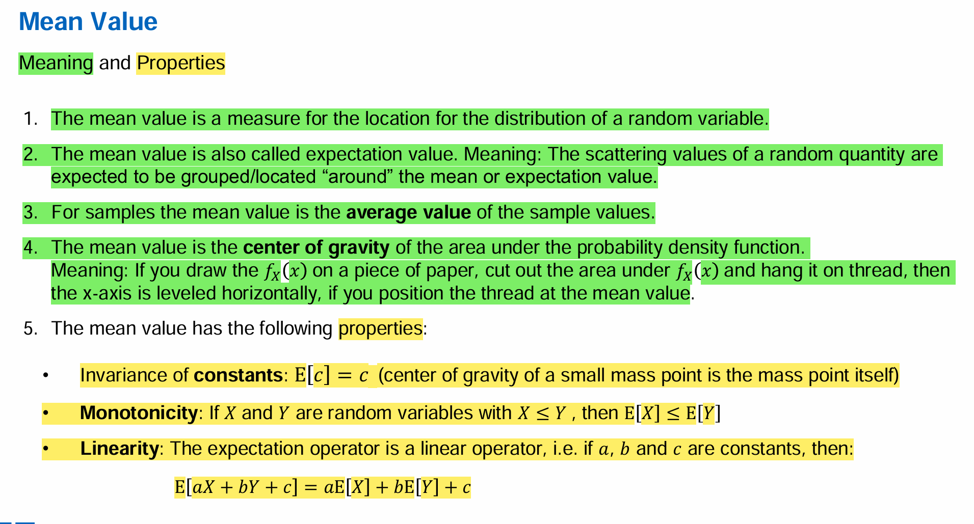
→ Mean Value / Expectation Value

! the central moment for the 1st Statistical Moment is always zero !

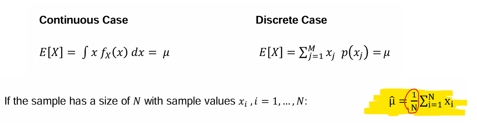
Define the term “Mean Value” and its Properties

What paramter characterizes the shape of the scatter in “Second statistical moment”

→ Variance / Standard Deviation

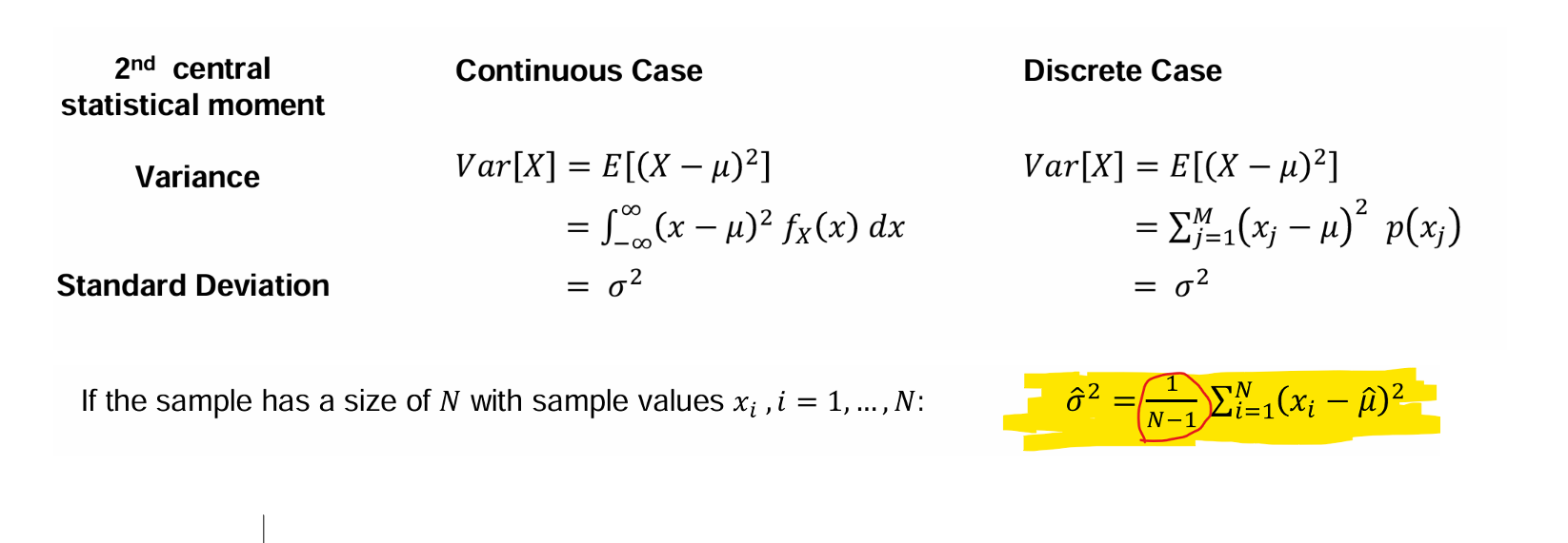
Define the term “Variance” and “Standard Deviation”

Variance = Measure the width of the distribution of a random variable, i.e. how far away from the mean value the sample values are. It has the unit of the square of the physical quantity of sampled data

Standard Deviation = Sqrt(Variance). It has the unit of the physical quantity of sampled data

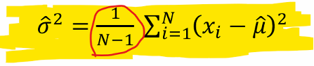
Where is the “N-1” in the dominator for Estimate Standard Deviation coming from ?

For calculating Estimate Mean Value = The set of 𝑁 samples has already been used

Afterwards, only “N-1” degrees of freedom left for determining other quantities (i.e. Estimate Standard Deviation)

What paramter characterizes the shape of the scatter in “Third statistical moment”

→ Skewness

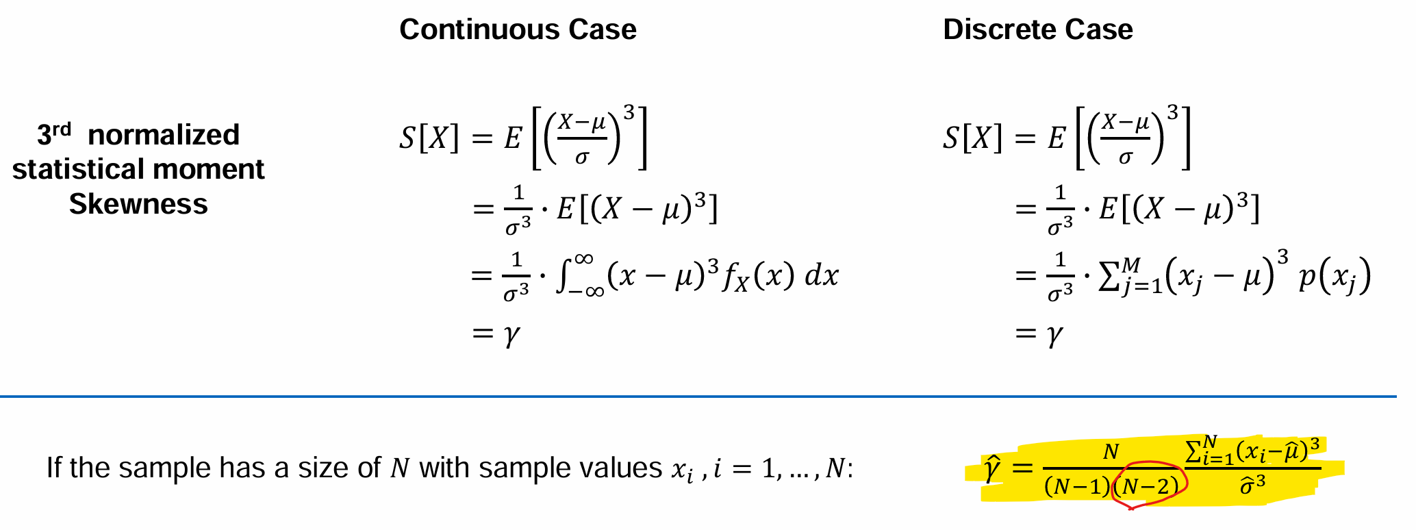
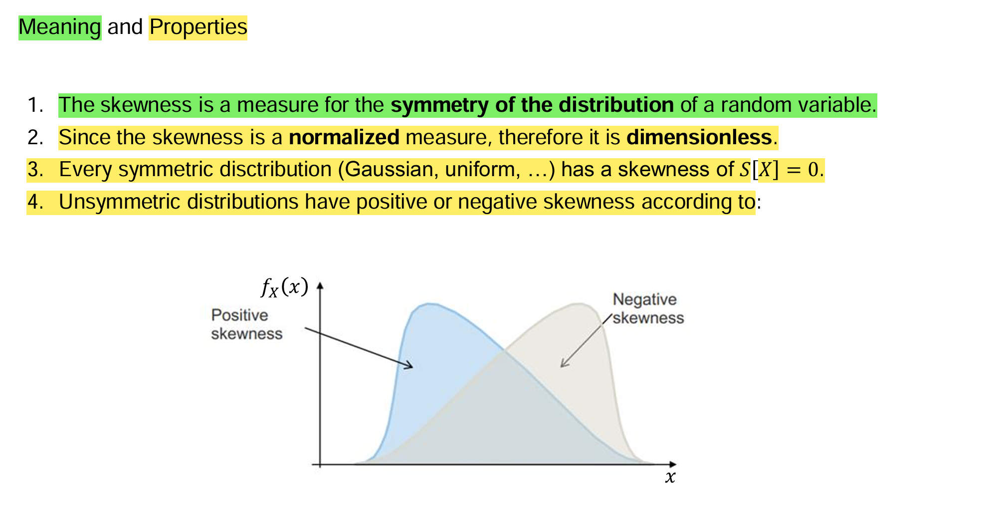
Define the term “Skewness” and its Properties

What paramter characterizes the shape of the scatter in “Fourth statistical moment”

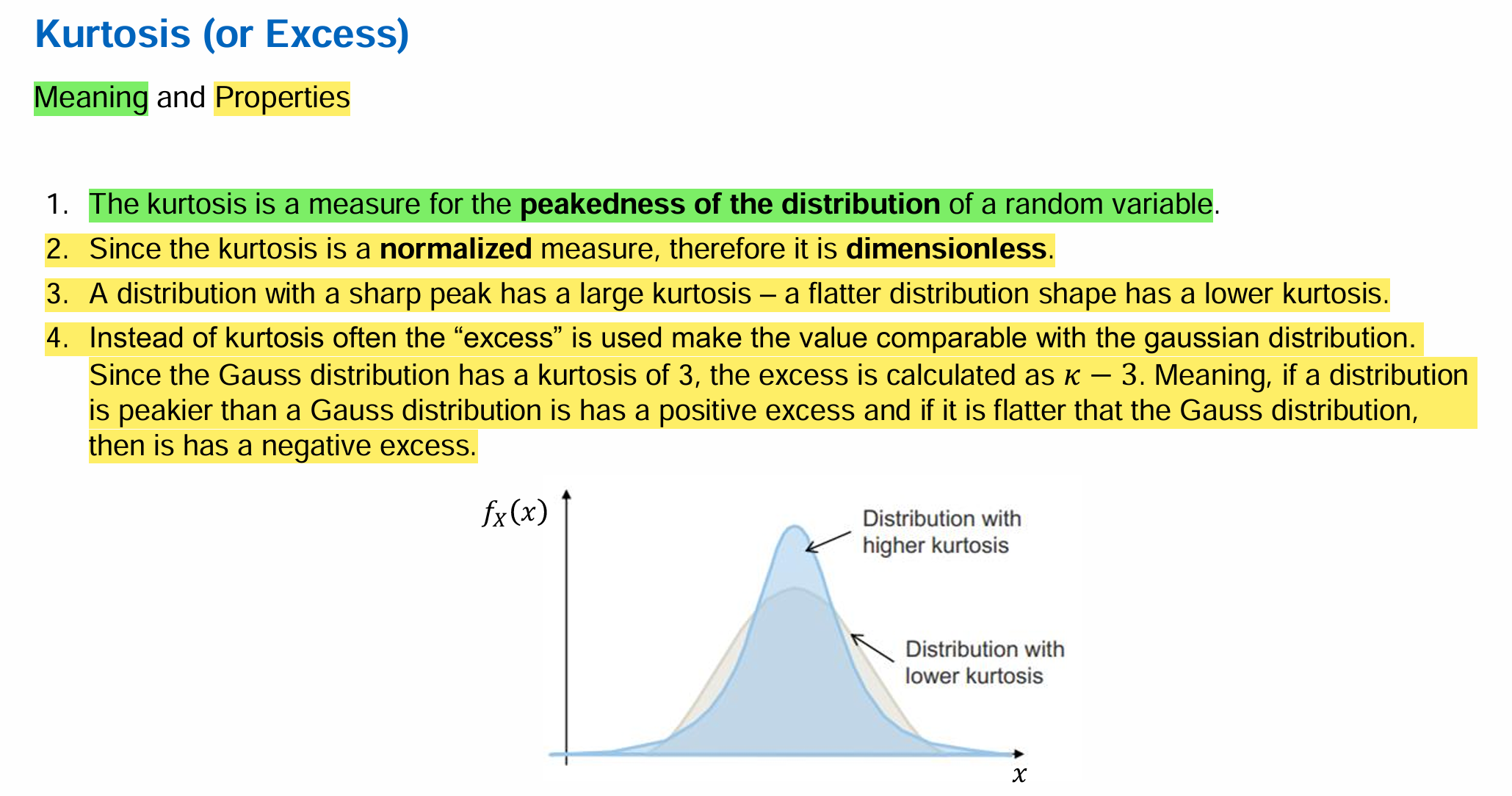
→ Kurtosis

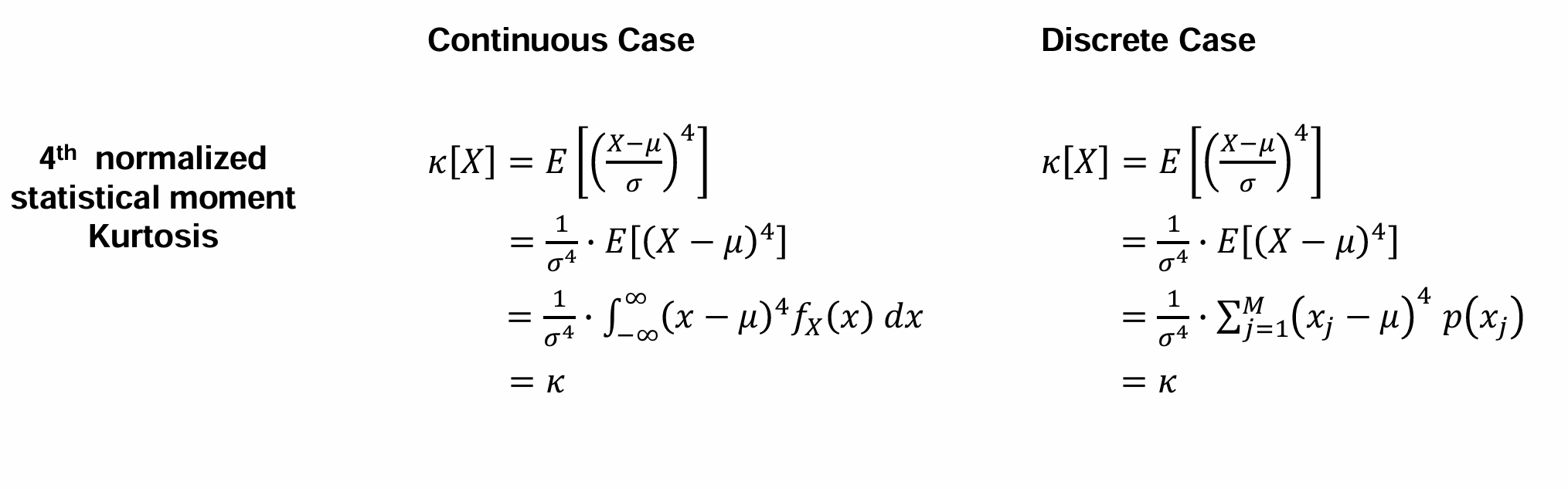
Define the term “Kurtosis” and its Properties

What paramter(s) characterizes the shape of the scatter in “Mixed Second statistical moment”

→ Covariance

The covariance is a measure for statistical relationship between two random variables.

→ Correlation coefficient

More common to use the normalized and therefore dimensionless than Covariance

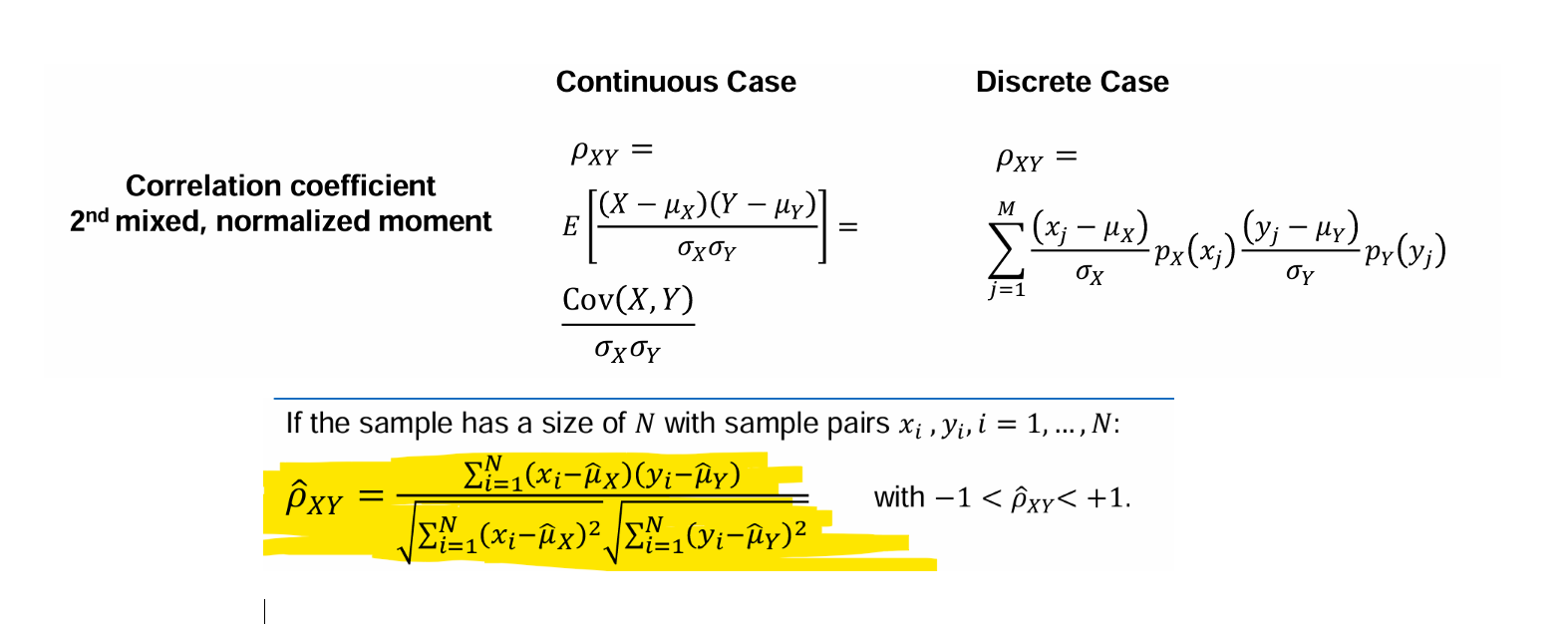
Define the term “Linear Correlation Coefficient”

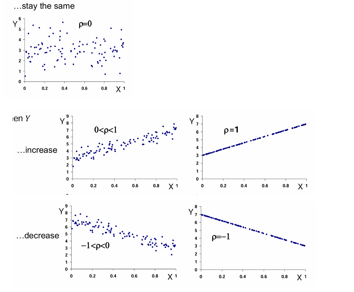
The linear correlation coefficient is a measure for the intensity of the linear statistical relationship between the random variables 𝑋 and 𝑌.

Example: If 𝑋 is increasing then 𝑌 tends to ..

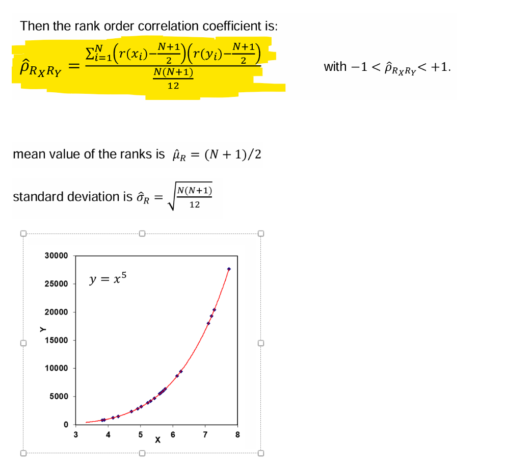
What does the “Spearman rank order correlation coefficient” measure ?

It’s a measure for the intensity of any non-linear, but monotonic relationship (dependency) between the random variables 𝑋 and 𝑌.

How is Sensitivity given by “deterministic variables” and “random variables” ?

For Deterministic Variables → given by the slope (derivative) of 𝑌 wrt. 𝑋_i ,

\frac{dY}{dX_{i}}

For Random Variables →by the slope (derivative) AND the width of the scatter of 𝑋_i

➔Both aspects are taken care by the correlation coefficient!

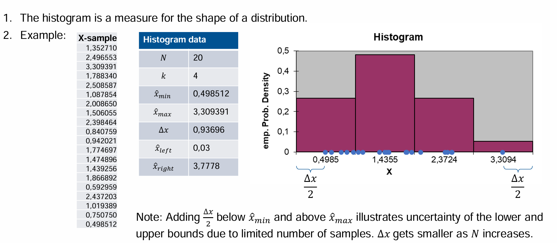
Explain step-by-step process of how to create a histogram

1. From the sample data derive the number of samples 𝑁, the smallest sample value \overline{x}_{\min} (sample minimum) and the largest sample value \overline{x}_{\max} (sample maximum) Please note: the minimum/maximum of the sample is NOT the minimum/maximum of the entire set. It is an estimate, hence the hat “^”

2. Using the number of samples 𝑁 determine a “good” number for the intervals. With: 𝑘 = 𝑟𝑜𝑢𝑛𝑑(min( sqrt(𝑁),10 ∙ log_10 (𝑁))

3. Divide the data range into 𝑘 intervals of equal width Δx = \frac{\overline{x}_{\max}-\overline{x}_{\min}}{k-1} such that \overline{x}_{\min} is the center of the left most interval and \overline{x}_{\max}

   is the center of the right most interval. This means the histogram ranges from \overline{x}_{left}=\overline{x}_{\min}-\frac12\frac{\overline{x}_{\max}-\overline{x}_{\min}}{k-1} to \overline{x}_{right}=\overline{x}_{\max}+\frac12\frac{\overline{x}_{\max}-\overline{x}_{\min}}{k-1}

4. Correct \overline{x}_{left} and \overline{x}_{right} if physical bounds are violated. E.g. if \overline{x}_{left} < 0 for a positive quantity set \overline{x}_{left} = 0

5. Count the “hits” 𝑛_𝑗 of the sample data in each interval with 𝑗 = 1,…𝑘. Devide the hits by the total number of samples 𝑁 and by the width of the interval Δx, i.e. p_{j}=\frac{n_{j}}{N\cdot\Delta x}

6. Plot the 𝑝_𝑗 versus 𝑥_𝑗, where 𝑥_𝑗 are the center of the intervals

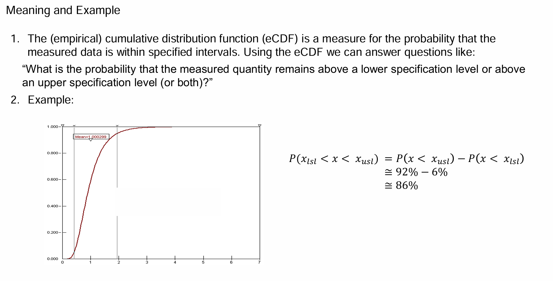
Explain step-by-step process of how to create a Empirical Cumulative Distribution Functions

1. Order the sample data in ascending order and note the order number of the sample data. I.e. the smallest sample value has the order number 1, the second smallest hast order number 2 and so on all the way up to order number 𝑁, for the largest sample value

2. Assign probabilities to the ordered sample values 𝑥𝑖 with 𝑖 is the order number as: P_{i}=\frac{i}{N+1} or P_{i}=\frac{i-0.3}{N+0.4}

3. Plot the (x_i, P_i)

What does the histrogram measure ?

What does the Empirical Cumulative Distribution Function measure ?