AP Stats Unit 2: Normal Distribution

Might not correspond to Unit 2: Exploring Two-Variable Data.

percentile

% of values that are less than or equal to a given value; i.e. the cumulative relative frequency

• “at Xth percentile” - not “in” - percentile is a location, not a bucket

calculating percentile:

• percentile = proportion from the left

• = (# of points less than or equal to)/(total # of points) * 100 (for a full #)

*for normal distributions, can use:

• normalcdf(lower: -10^99, upper: value (or z-score of value), mean: mean (or 0), SD: SD (or 1))

• = proportion * 100

• = percentile

proportion

percentile but as a fraction

= percentile/100

= %/100%

cumulative relative frequency

adding up all the relative %s before that data point

= to the percentile (as a proportion from the left)

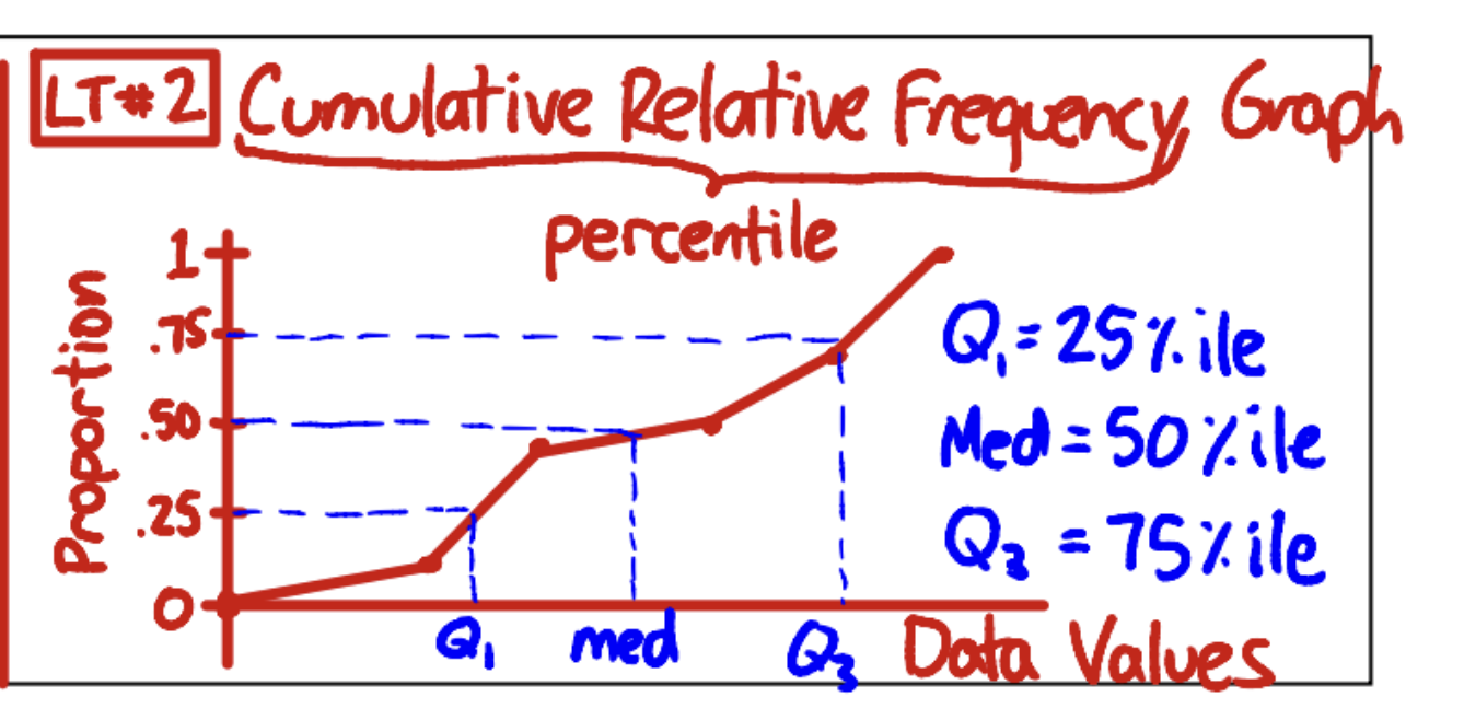
GRAPH: cumulative relative frequency

graphing cumulative relative frequency:

• x-axis: data value

• y-value: proportion (on a 1.0 scale)

• use straight lines between the points known/given since we don’t know the behavior of the data between the points

estimating using a graph:

• guess using the graph, linearly, where the line’s y-value would line up for that x-value

important notes:

• median: x-value with 0.5 y-value

• Q1: x-value with 0.25 y-value

• Q3: x-value with 0.75 y-value

INTERPRETATION: cumulative relative frequency

PERCENTILE% of [specific subjects] have a [measured variable] equal to or less than [value], the [value] of the [subject that the percentile is of]

z-score

= (value - mean)/SD

“standardized score” that allows for comparison to:

• a standardized curve if you know the distribution of the data (e.g. a normal distribution)

• the dataset overall to know much MORE something is in comparison to the mean/variability of the original

INTERPRETATION: z-score

the [measured variable] of the [specific subject that has the z-score] is [z-score] standard deviations below the mean of [mean value & context]

effects of +- a constant to all values in a dataset

• shape: no change

• center: +- that constant

  • ex: mean = old mean +- constant

    • all of them got +- constant, so total we had a change of n*+-constant

    • finding the mean → must divide by /n, so the change also gets divided:

      • change = n*+-constant

      • n*+-constant/n = +-constant → this is the final change

  • ex: median = old median +- constant

    • obviously, bc all values had the constant +-

• variability: no change

effects of */ a constant to all values in a dataset

• shape: no change

  • stretching in any way → does NOT change the shape itself, but only the scale of of the shape (because the distribution of the points themselves doesn’t change)

• center: */ that constant

  • ex. mean = old mean */ constant

    • old mean = (total dataset)/n

    • new dataset: constant*(total dataset)

    • new mean = constant*(total dataset)/n = constant*(old mean)

  • ex. median = old median */ constant

• variability (SD): */ that constant

  • because distance between the distance */ constant as well

  • variance: */ constant² — “Since we multiplied the SD by x, variance was multiplied by x²”

shape, mean, & SD of a z-score distribution

• shape: same

• mean: 0

• standard deviation: 1

because:

• z-score is a linear transformation on the values: (value - mean)/SD

• -mean: mean becomes 0, SD stays the same

• /SD: mean is 0/SD = 0, SD becomes 0

• *throughout all changes, shape stays the same

density curve

graphical representation of the probability distribution of a numerical variable (may be continuous and is smoothest that way, but could be discrete)

features:

• total area = 1

  • other “area” rules apply (represents #/density of points in that area); think of it like a “smoothed out histogram”

• *this is essentially the integral of the function (x, f(x)) if you just drew the curve tops. the area below it = the integral of this function (which is how the calc would do it)

telling if skew:

• skewed left: many low-probability points to the left (tail off to the left)

  • mean < median

• skewed right: many low-probability to the right (tail off to the right)

  • mean > median

• symmetric: poitns are distributed about evenly around a mean in the center

  • mean ~= median

mean:

• 50% of the area on one side

• 50% of the area on the other side

normal distribution

a common curve that appears in all of nature/the world; when the density curve is perfectly symmetric & follows the empirical rule

• N(mean, SD): graph of normal distribution with mean & SD

• iff empirical rule → normally distributed & the other way around

proving something is normal:

• empirical rule is similar to the real %s between SD’s

• use normalcdf(value) and check if the given proportion of that value is similar to the calculated normal proportion

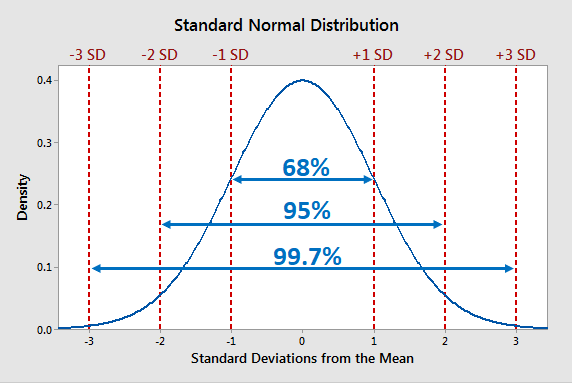
empirical rule (68-95-99.7 rule)

68% of data is 1 SD away from mean in either direction; 95% of data is 2 SD away from mean in either direction; 99.7% of data is 3 SD away from mean in either direction

• applies only for normal distributions

usage:

• can be used to estimate %s without a calc/z-table, particularly if the values lie on perfect SD counts (or almost perfect; the further they get from these perfect SD counts, the worse the approx. becomes, bc we assume it’s linear but it isn’t)

• can be used to “guess” about how many SD’s or %s a data point should be between (given one or the other)

Calculating Proportion from a Boundary Value (specific x) — Normalcdf

GRAPH & PROCESS:

• must draw curve — either original or standardized ok

  • (standardized needs you to INPUT the z-score)

  • label: mean, value, N(mean, SD)

  • shade: area of interest

• *CALCULATE THE Z-SCORE REGARDLESS

  • always need to do this, even if you don’t use it in the final calculation

• *NEED LABELS on functions (lower, upper, mean, SD)

  • mean, SD can be the greek letters or just the words

original version:

• curve with N(mean, SD) given and then:

  • label mean

  • label cutoff value (literally just the value you have)

  • shade area that you are calculating

• label all of the calculations with: upper = actual value, mean (μ) = actual, SD (σ) = 26)

• = proportion

• → area (* 100% of proportion, round to tenth of a percent)

standardized version:

• curve with N(0,1) and then:

• label 0

• label the cutoff value

• shade the area that you are calculating

• normalcdf(lower: NUMBER (-1*10^99), upper: NUMBER, mean: 0, SD: 1)

• = proportion

• → area (* 100% of proportion, round to tenth of a percent)

CALCULATION:

• x is known, proportion/percentile/area is not

• normalcdf(lower, upper, mean, SD)

Calculating Boundary Value (specific x) from a Proportion — invNorm

GRAPH & PROCESS:

• must draw curve — either original or standardized ok

  • label: mean, N(mean, SD)

  • *also label value (specific x), BUT label with an “x”

  • shade: area of interest

• *CALCULATE THE Z-SCORE

  • *can be done in 2 ways:

  • 1. before you get the actual value, use the standardized method → automatically returns the z-score for you

    • invNorm(area: proportion, mean: 0, SD: 1) = z-score

  • 2. use the original method → manually calc z-score afterward

• *NEED LABELS on functions (lower, upper, mean, SD)

  • mean, SD can be the greek letters or just the words

CALCULATION:

• proportion/percentile/area is known, x is not

• invNorm(area, mean, SD, area of interest (left/right/center))

• notes on left/right/center:

  • left: aka percentile from left, proportion from left, or area from left

  • right: aka percentile from right, proportion from right, or area from right

  • center*: usually not used until we get to confidence intervals - helps us find the boundary values for a confidence interval of 95%, for example; would give us the values on the low and high end if we “fill in” 95% in the middle

    • equivalent to finding 2.5% on left & 2.5% on the right (or 97.5% on the left)