BioImaging Subjects 1 & 2

Signals

math functions of 1+ ID variables, model physical processes

Image (2D)

function of 2 ID real valued variables (pixels)

visual representation of 2D signal

Delta/Impulse Function

models a point source (char resolution)

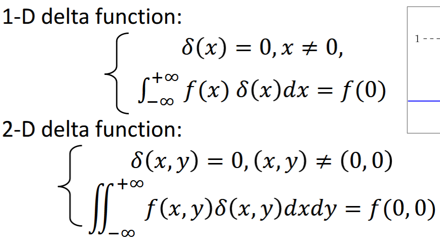
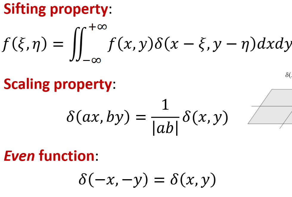
Delta Function Properties

Shift, Scale, Even

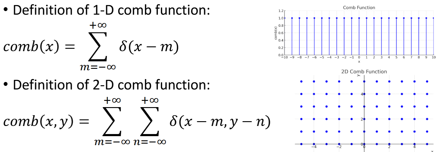
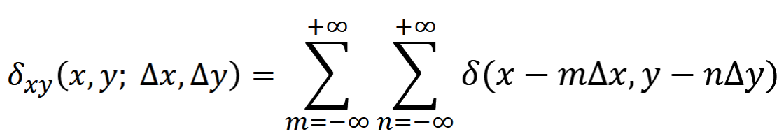
Comb Function

shows pixel grid

Sampling

converts continuous signals to discrete signals. Summations

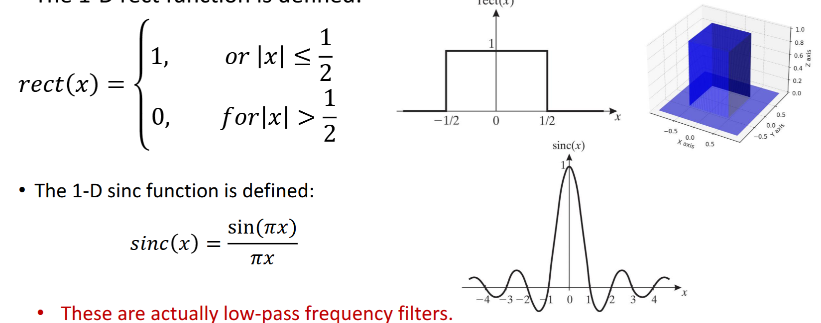
Rect and Sinc Functions

Low pass filters, fourier transforms of each other

Separable Signals

most medical images, 2D functions that can be reduced to 1D operations. f(x,y)=f(x)*f(y)

System

transformation 𝓈 of input signal f to output signal g.
𝓈 = characterization of the system, blurring function

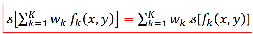
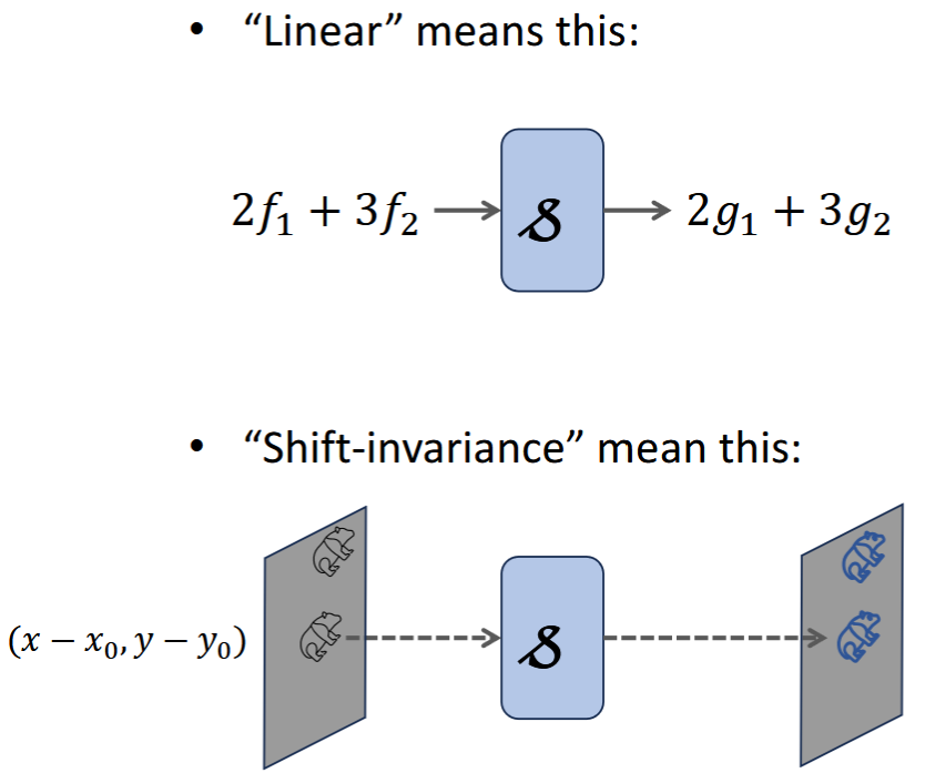
Linear System

• Scaleable - input x C = output x C

• Superposition - 2 inputs => output = output1+output2

• most medical systems

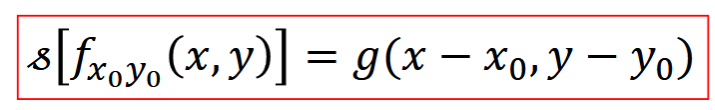
Shift Invariant System

translation of input => same translation of output

LSI System

Linear and shift invariant system, most medical

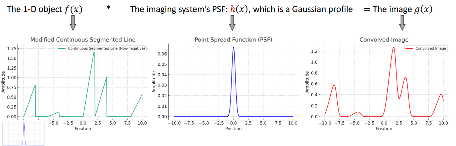
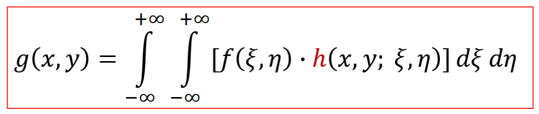
Point Spread Function (PSF)

output of system to a delta function, h, superposition integral, defines system, mostly gaussian profile

for LSI: g(x,y)=h(x,y)*f(x,y)

*= convolution operator

LSI System Connections

1. Cascade: h=h1*h2

2. Parallel: h=h1+h2

3. Associativity: h2*[h1*f]=h1*[h2*f]=[h1*h2]*f

4. Commutativity: h1*h2=h2*h1

5. Distributivity: g(x,y)=h1*f+h2*f=(h1+h2)*f

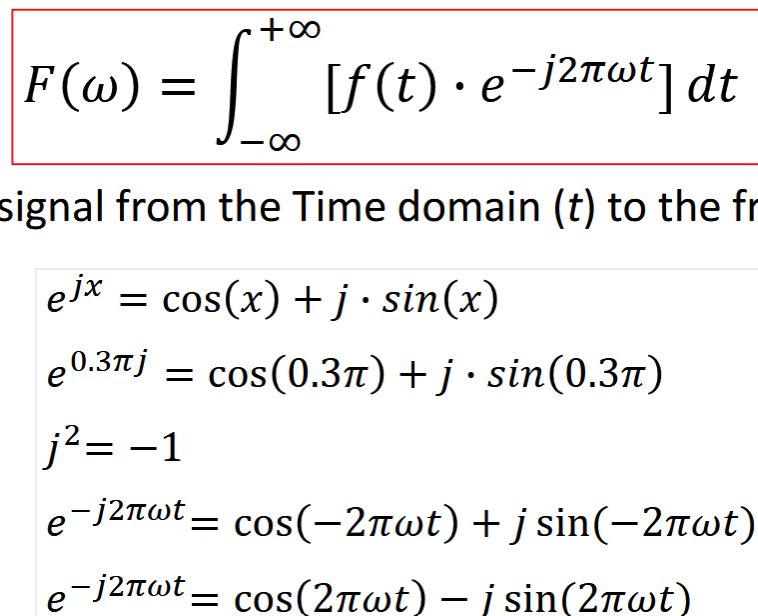
Fourier Transform

transforms signal from time domain to frequency domain

can be used to analyze spectral components, sep consider action of LSI at each sinusoidal frequency

F(u,v) = spectrum of f(x,y), sinusoidal composition at dif frequencies

Spatial vs. Frequency Domain

spatial - normal image, pixel coordinates and intensity values

frequency - FFT based frequency components, magnitudes and phases

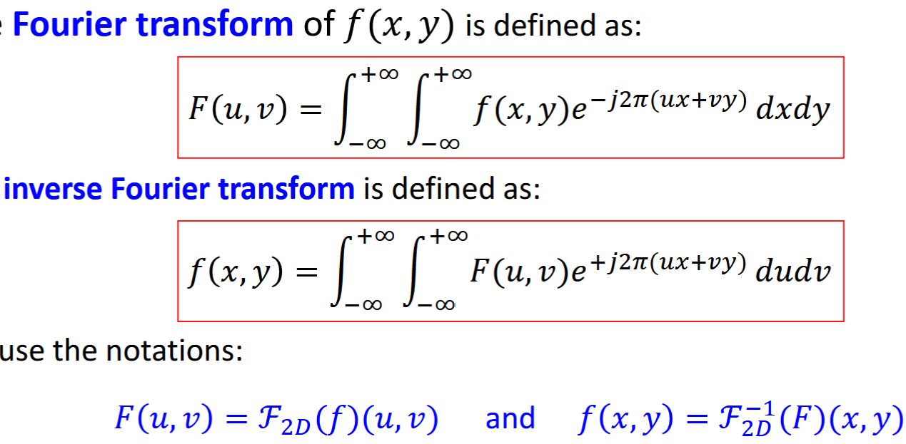
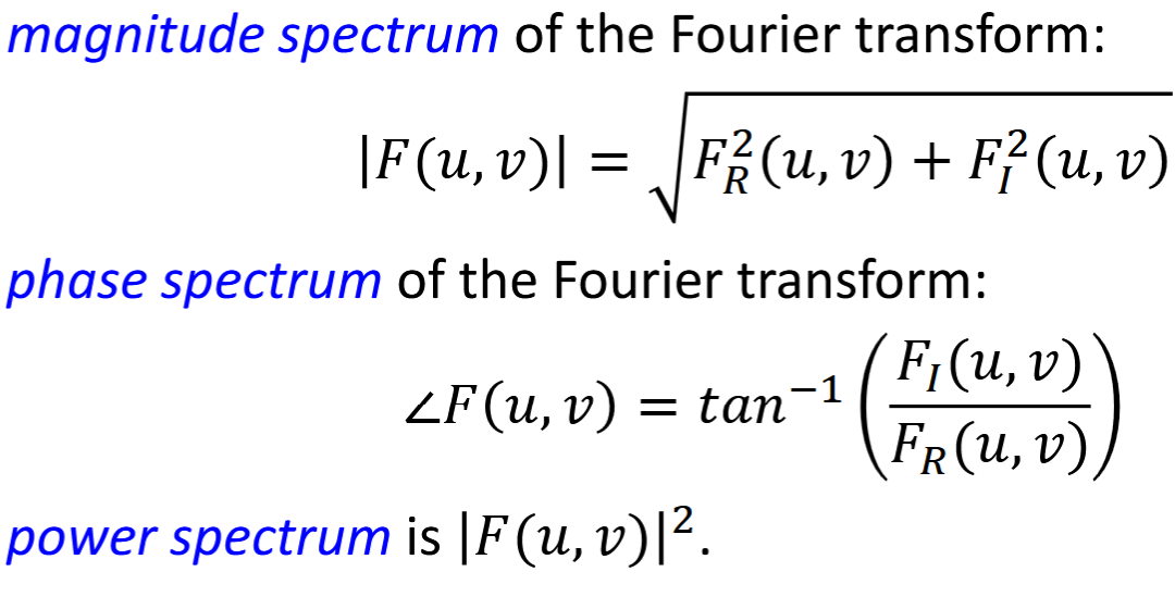
Fourier Transform Spectrums

f(x,y) real valued, F(u,v) complex valued

FT of delta function = 1

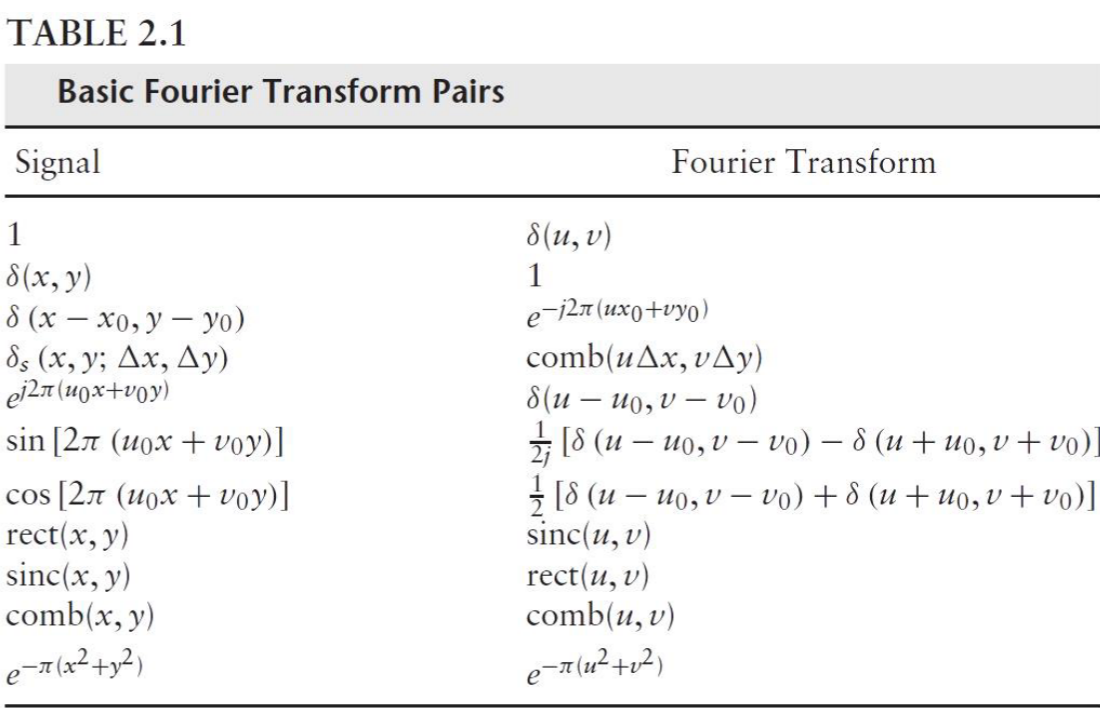
Fourier Transform Pairs

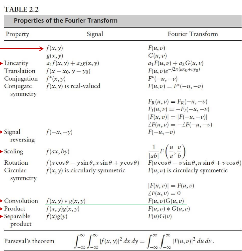
Fourier Transform Properties

Spacial Frequencies : Image Quality

• LPF (low frequencies stay) - most of the image, blurred

• HPF (high frequencies stay) - sharp edges of the image

• slow signal variation = low frequencies

• fast signal variation = sharper features, high frequencies

• req high spatial frequency for fine structure high quality

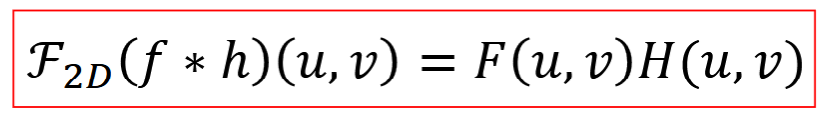
Convolution Theorem

convolution in spatial = multiplication in frequency

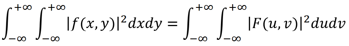
Parseval’s Theorem

total energy of a signal in the space domain = total E in frequency domain
FT & inverse are energy preserving

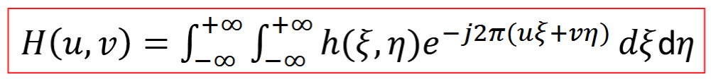
Transfer Function

Fourier transform of PSF, H(u,v)

optical transfer function

G(u,v)=H(u,v)F(u,v)

Cutoff Frequency

limited frequency bandwidth

filtering with it → signal smoothing (higher spatial frequencies eliminated via imaging, c1>c2)

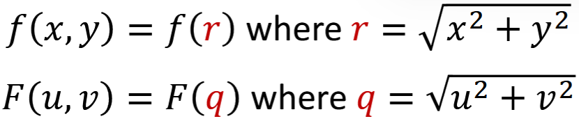
Circularly Symmetric Signals

f_theta(x,y) = f(x,y) for every theta

Fourier transform is also circularly symmetric

Hankel Transform

F(q)= H { f(r) }

Fourier transform of circularly symmetric 1 | 2D signals, including Gaussian

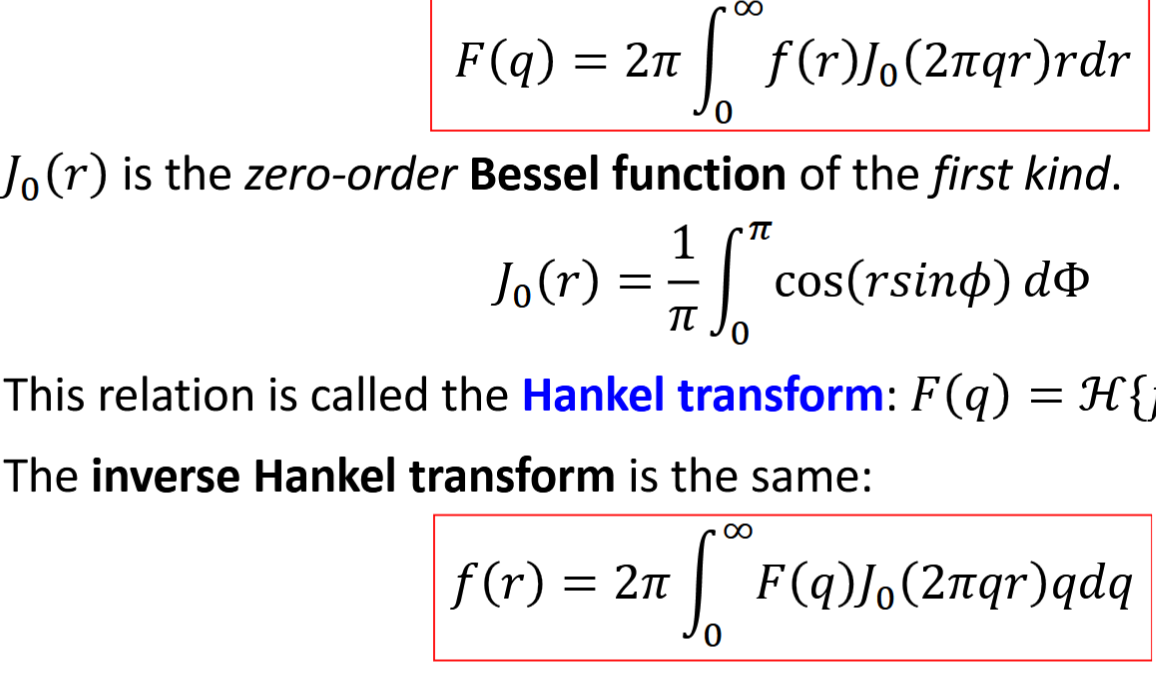
Image Quality Evaluation

contrast, resolution, noise (SNR), sampling (nyquist), artifacts, distortion, DA (sensitivity and specificity)

Image Quality Importance

image internal structures and functions of the patient body to diagnose abnormal conditions, guide therapeutic procedures, monitor the effectiveness of treatment

quality = degree to which an image allows accomplishment of these goals

Contrast

• dif btwn image intensity of object and background, result of inherent object contrast within body

• need high contrast for abnormality detection, preserve true object contrast

• quantified with periodic signal with modulation, modulation (depth). mf<1, no contrast if mf=0

• mg = modulation/contrast of the image = mf [H(u0,0)/H(0,0)]

Sinosoidal Object

f(x,y) = A + Bsin(2 pi u0 x)

fmax = A+B fmin=A-B mf=B/A

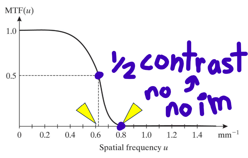
Modulation Transfer Function

• MTF, mg/mf = |H(u,0)|/H(0,0)

• quantifies degradation of contrast as function of spatial frequency. 0 <= MTF(u) <= MTF(0) = 1

• better MTF = greater area under the curve

• summed for subsystems by multiplication, overall is always less than single

Local Contrast

difference btwn target and background

Contrast Mechanism

type and principle of contrast

• CT - x-ray absorbtion coefficient of tissue

• MRI - concentration of H atoms in tissue

• Raman spectroscopy - chemical bond vibration

• Fluorescence microscopy - fluorescence emission from fluorescent molecules

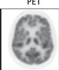
Resolution

• capability to accurately depict two distinct events in space/time/frequency as separate corresponding to the spatial/temporal/spectral resolution

• PET has high contrast and poor spatial resolution

• can be quantified by the period of sinusoidal input. resolution = period of sine at 1/uc

Full Width at Half Maximum

full width of LSF/PSF profile at half the maximum value [mm], equals resolution

summed in square: R = sqrt(R1² + R2² +…+Rk²), heavily effected by large terms

Bar Phantom

tool to measure resolution, image through the system to eval resolution

density of lines = line pairs per mm [lp/mm]

Noise

any random fluctuation, unwanted char, numerical outcome of statistically random events

image quality decreases as noise increases over the signal

amplitude rep by SD, power rep by variance, a = average intensity, # of photons

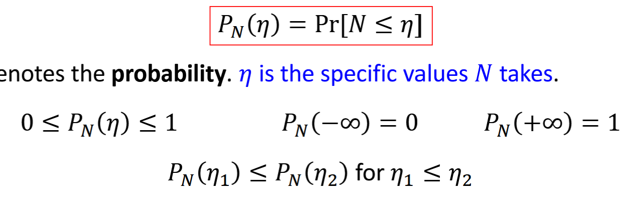
CDF

cumulative distribution function

N (random variable) = number for random event, mathematically described by CDF

Pr(*) = probability; n = specific values of N.

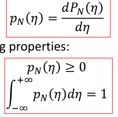
PN(n) for continuous random variable = integral from - infinity to n of pN(u) du

pdf

probability density function, gaussian and uniform

specifies continuous random variable. sums as convolution products

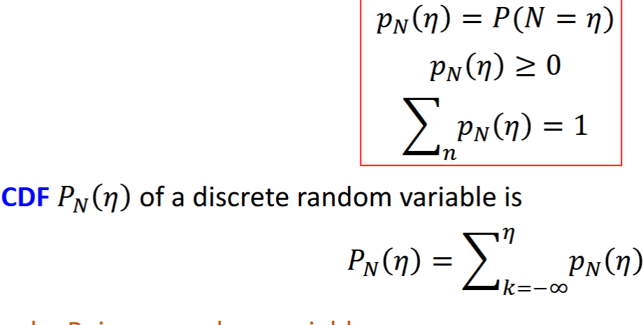
pmf

Probability mass function, discrete random variables (N discrete)

poisson

Stats for Noise

• expected value = mean = uN E[N] = integral of n times pN(n) dn. sums

• variance = oN² = Var[N] = E[(N-uN)²] = integral of (n-uN)² times pN(n) dn. sums

• standard deviation = sqrt(variance)

• integrals for continuous, summation for discrete

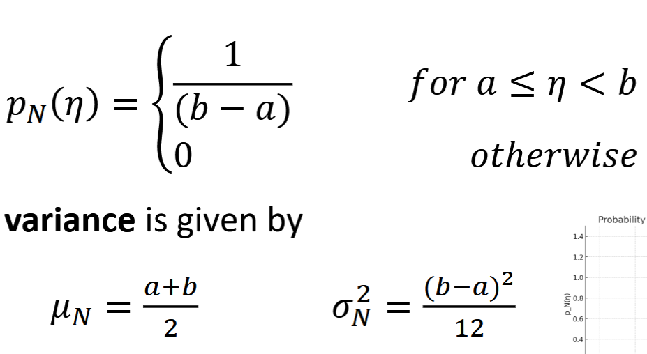
Uniform Random Variable

continuous, specific pdf

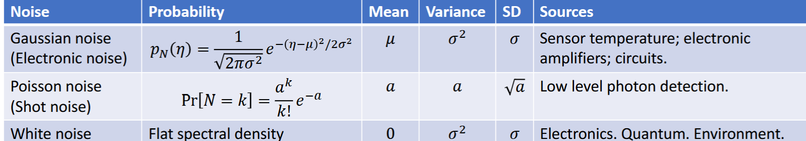
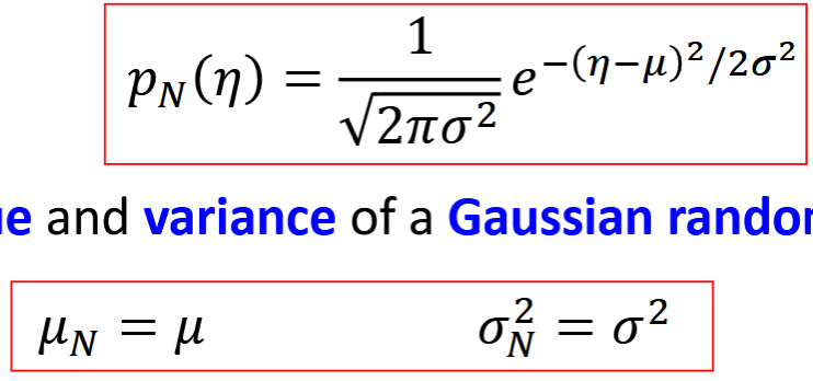
Gaussian Random Variable

continuous, natural to model noise with, based on pdf

Sensor temperature; electronic amplifiers; circuits

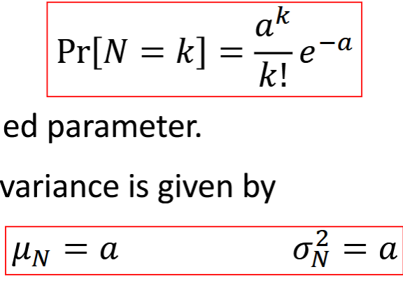
Poisson Random Variable

discrete, based on pmf, low level photon detection noise, a>0

graph has tail to the right. shot noise

White Noise

equal intensity at different frequencies, constant power spectral density, Electronics. Quantum. Environment.

mean = zero, constant variance, serially uncorrelated Cov[N(t),N(s)]=0 for t not equal s

SNR

signal to noise ratio. prefer higher (output g more accurate to input f)

describes relative str of signal f with respect to noise N

blurring process reduces, higher noise reduces

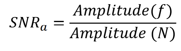
Amplitude SNR

• frequency amplitude / noise amplitude

• Poisson = photons per unit area / standard deviation. SD = sqrt(mean) SNRa=sqrt(mean). more photons = higher SNR = higher im qual

• SNR (in dB) = 20log(SNRa)

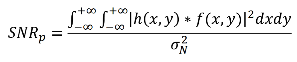
Power SNR

• signal power / noise power

• white noise: noise power = variance, mean = 0

• SNR (in dB) = 10log(SNRp)

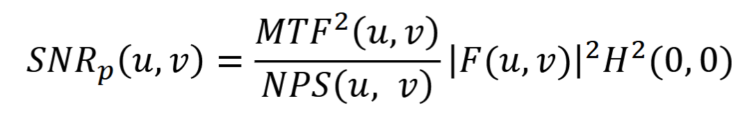
Frequency Dependent Power SNR

nonwhite noise, provides relation btwn contrast, resolution, noise, and image quality. up MTF = up im qual

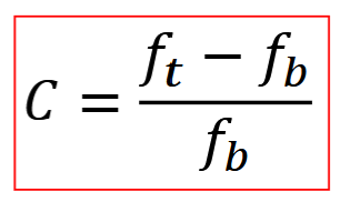
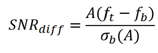
Differential SNR

A = area, ft = average image intensity within A, fb = average image intensity within A of background

SDn(A) = standard deviation of image intensity vals over area of the background

SNR (in dB) = 20log(SNRa)

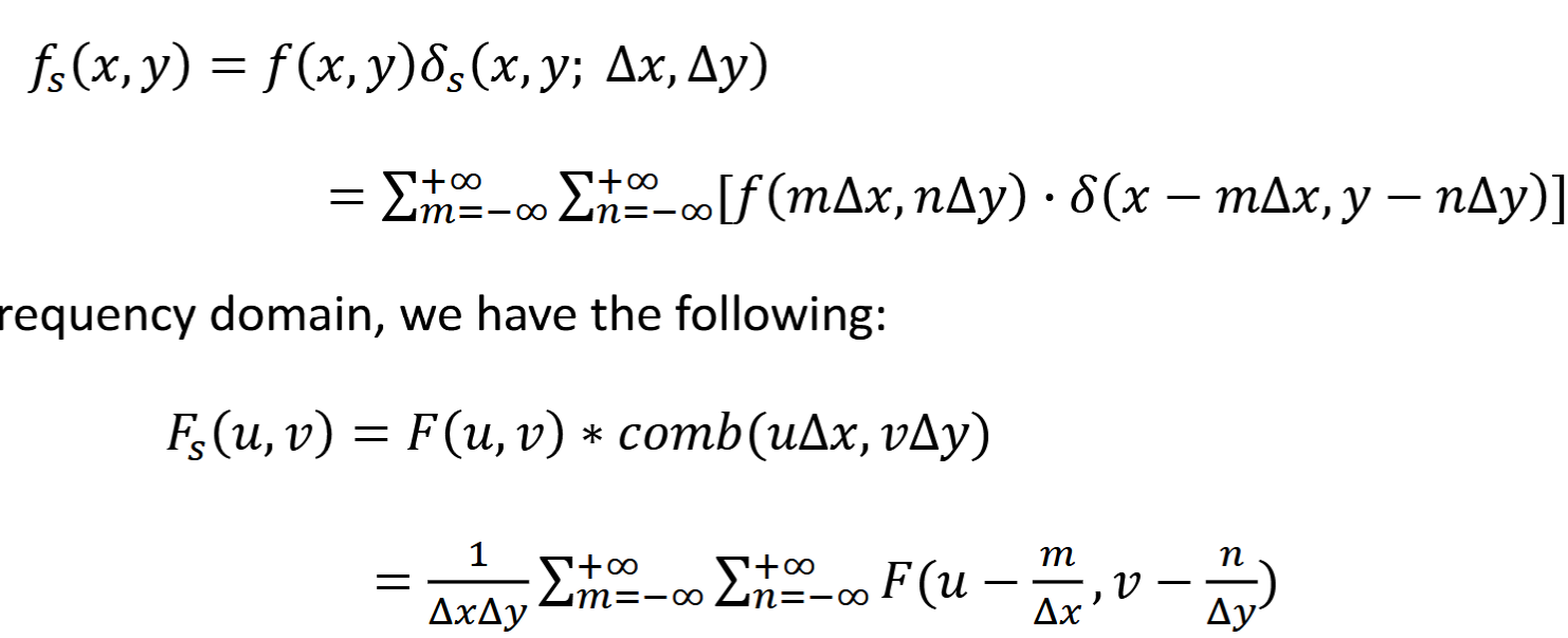
Sampling

∆𝑥 and ∆𝑦 are the sampling periods; 1/∆𝑥 and 1/∆𝑦 sampling frequency

𝑓𝑑 (𝑚, 𝑛) = 𝑓 (𝑚∆𝑥, 𝑛∆𝑦) ∆𝑥 <= 1/2U and ∆𝑦 <= 1/2V

Aliasing

artifact from low sampling, new high frequency patterns where none should exist

Nyquist Sampling Theorem- avoid aliasing by ∆𝑥(max) = 1/2U and ∆𝑦(max) = 1/2V. U=u0

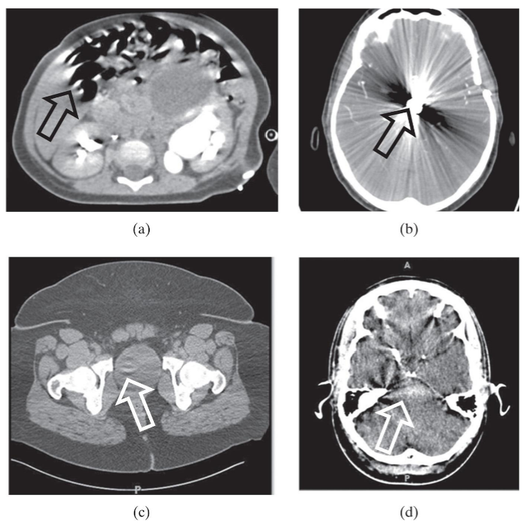
Artifacts

features of an image that do not represent valid anatomical or functional information. obscure

a = motion, b = star from metal, c = detectors out of calibration, d = xray beam hardening

Distortion

inability of medical imaging system to give accurate impression of shape, size, or position of object
CT - dif size look same from dif distance from x-ray source. identical look different due to orientation

Accuracy

• conformity to truth (free of error), clinical utility

• in context of diagnosis, prognosis, treatment planning, treatment monitoring

• quantitative accuracy and diagnostic accuracy

Quantitative Accuracy

numerical vals of given anatomic or functional image feature

error from bias (systematic reproducible difference, can be corrected) or imprecision (noise and random measure-measure variation)

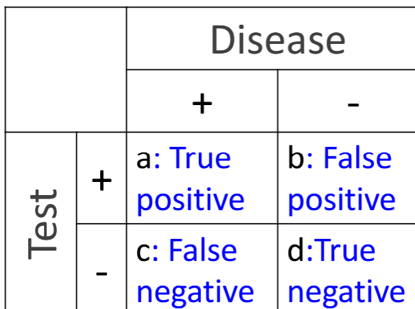
Sensitivity

true positive fraction, fraction of patients with disease who the test calls abnormal

a/(a+c)

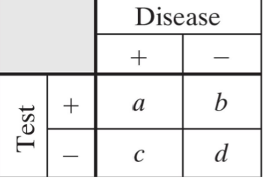
Specificity

true negative fraction, fraction of people without disease that the test calls normal

d/(b+d)

Diagnostic Accuracy

fraction of patients that are diagnosed correctly. max by max sensitivity and specificity

(a+d) / (a+b+c+d)

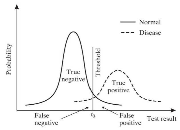
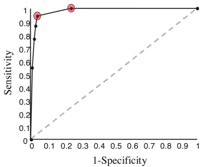
ROC Curve

lower threshold increases sensitivity and decreases specificity
plot of sensitivity (y) vs 1-specificity (x)

Prevalence

PR = (a+c) / (a+b+c+d) influences PPV and NPV

PPV = a / (a+b) called abnormal and have disease NPV = d / (d+c) called normal don’t have disease