unit 2 economics

12th grade ap economics

law of demand

- inverse relationship between price of good and quantity demanded by consumers
- P↑ = Qd ↓
- P↓ = Qd ↑

law of demand explanations

- law of diminishing marginal utility: bc utility goes down as you consume, you must lower prices
- income effect: as prices increase, consumers consume less bc of income constraint
- substitution effect: as price increase, consumers buy less bc of substitutes

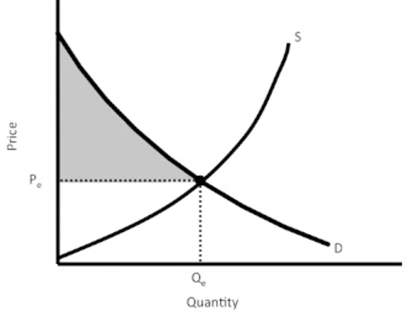
consumer surplus

difference between the price that a consumer is prepared to pay and the actual price paid

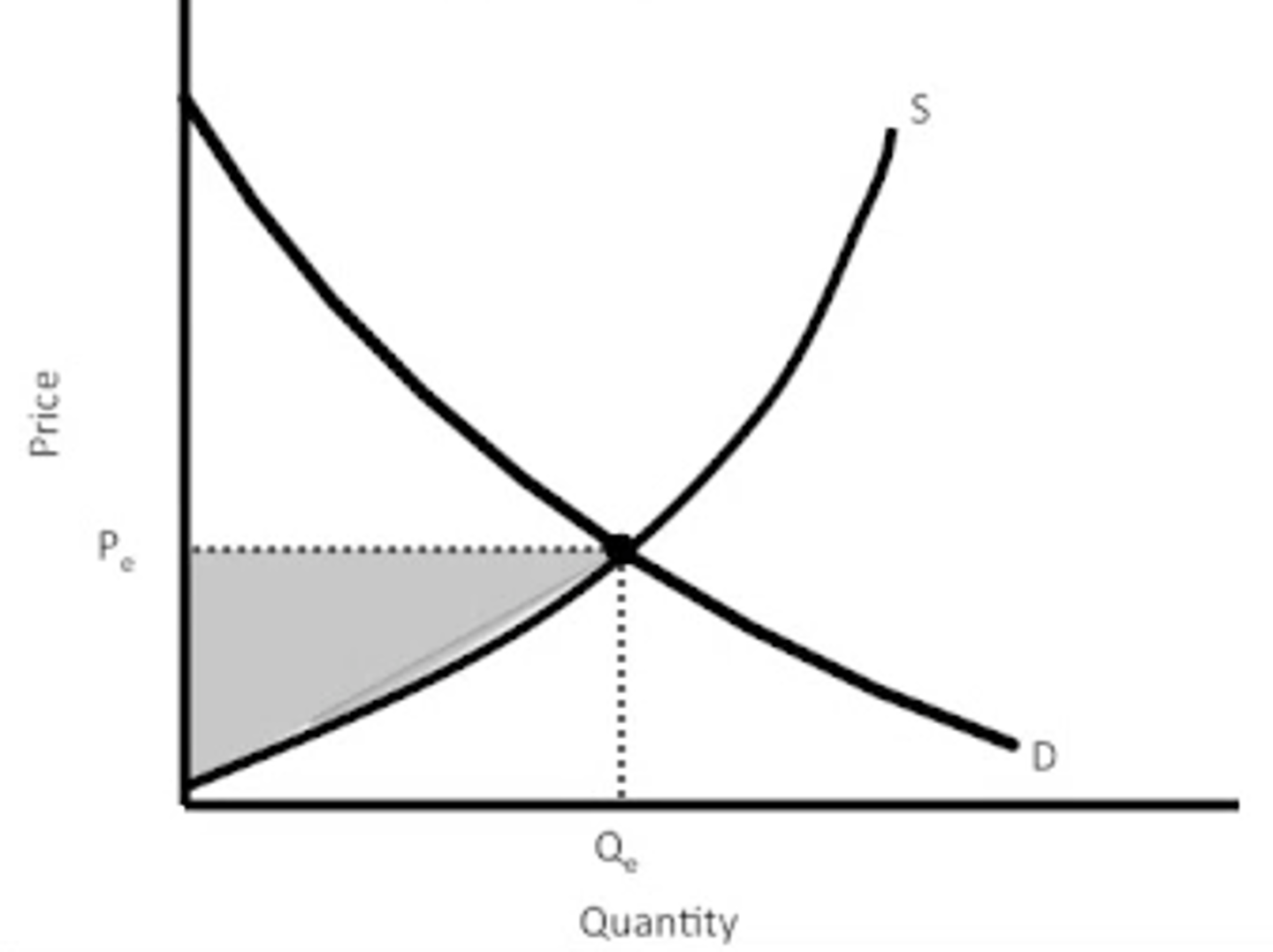
producer surplus

difference between the price that a producer is prepared to offer and the actual price charged

determinants of demand

- Price of related goods: substitute or complements
- Outlook: expectations
- Income: normal or inferior
- Number of buyers
- Taste: attitudes, advertising

change in quantity demanded

- price change
- movement along demand curve

change in demand

- something other than price changed
- shift of demand curve

substitute goods

- direct relationship
- Px↑ = Dy↑

complement goods

- inverse relationship
- Px↑ = Dy↓

normal goods

- direct relationship
- income↑ = D↑

inferior goods

- inverse relationship
- income↑ = D↓

determinants of supply

- Size of industry
- Price of related product lines that share same resources
- Input costs
- Government actions
- Outlook
- Technology

change in quantity supplied

- price change
- movement along supply curve

change in supply

- something other than price changed
- shift of supply curve

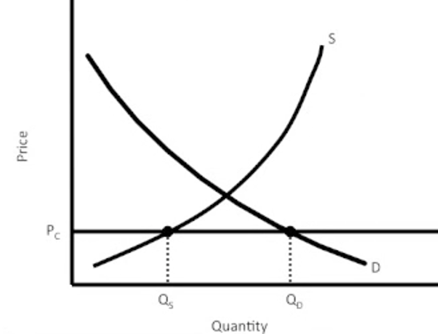
price ceilings

- below equilibrium
- shortage
- protect consumers
- cap on price/price cannot go up to equilibrium (maximum price allowed to charge)

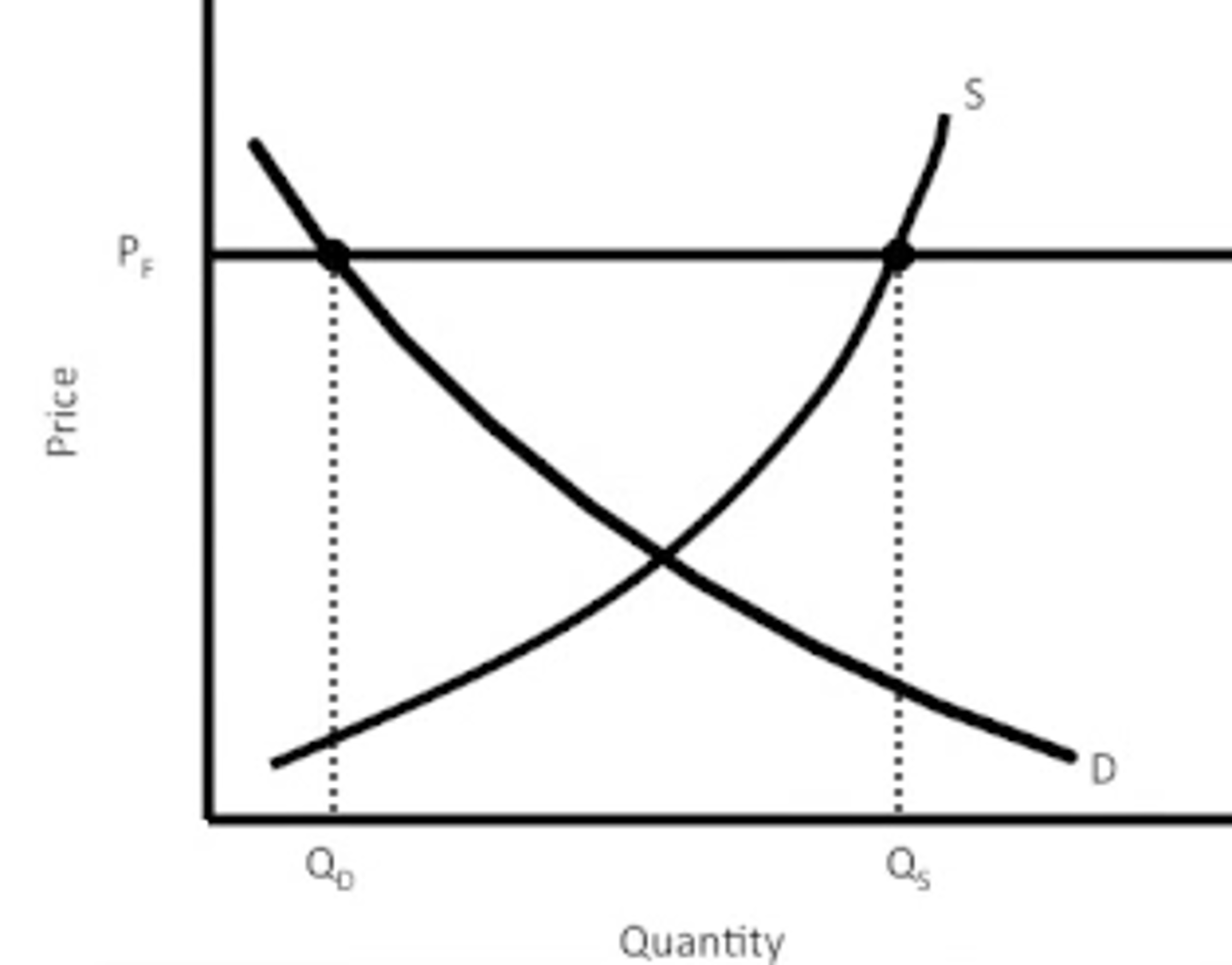
price floors

- above equilibrium
- surplus
- protect producers
- minimum price buyers are expected to pay

elastic

- quantity demanded/supplied is sensitive to price changes
- many substitutes
- P↑ = TR ↓ (inverse relationship)
- MR = positive

inelastic

- quantity demanded/supplied is not sensitive to price changes
- little to no substitutes
- P↑ = TR ↑ (direct relationship)
- MR = negative

price elasticity of demand (PED)

- coefficient test
- perfectly elastic = ∞
- relatively elastic = greater than 1
- unitary elastic = 1
- relatively inelastic = between 0 and 1
- perfectly inelastic = 0

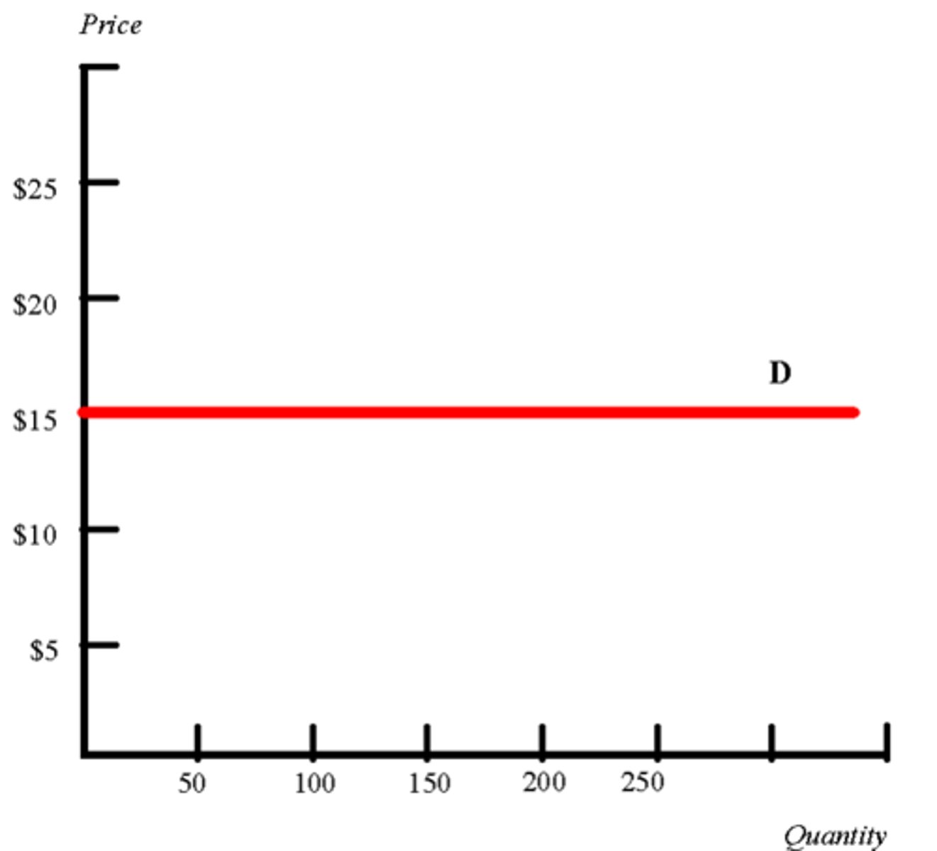
perfectly elastic

horizontal line

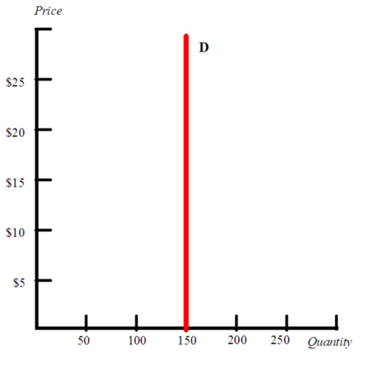
perfectly inelastic

vertical line

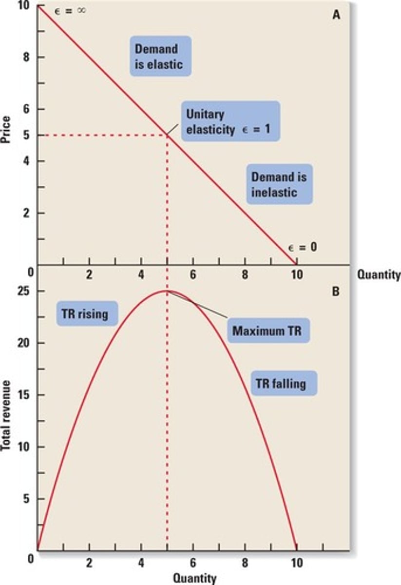
total revenue test

- multiply price by quantity
- elastic: P↓ = TR↑ (inverse relationship)
- inelastic: P↑ = TR↑ (direct relationship)

price elasticity of supply (PES)

cross price elasticity

- how the price of a good affects the demand of another good
- substitutes = positive (Px↑ = Qy↑; direct relationship)
- complement = negative (Px↑ = Qy↓; inverse relationship)

income elasticity

- how changes in income affects changes in demand
- normal good = positive
- inferior good = negative

incidence of tax

- burden on consumer: inelastic demand, elastic supply
- burden on producers: elastic demand, inelastic supply
- elastic demand: largest DWL, lowest tax revenue
- inelastic demand: lowest DWL, largest tax revenue

shortage

- quantity demanded > quantity supplied
- results in higher prices

surplus

- quantity demanded < quantity supplied
- results in lower prices

D↑, S↓ (double shift)

P↑, Q?

D↑, S↑ (double shift)

P?, Q↑

D↓, S↑ (double shift)

P↓, Q?

D↓, S↓ (double shift)

P?, Q↓

double shifts in demand and supply

- inverse D and S = price agrees with D and quantity is indeterminate
- direct D and S = quantity agrees with S and price is indeterminate