week 4 - model evaluation + hyper parameter tuning - need for model validation methods

recap: supervised learning

• model : form of function that we learn - characterised by free parameters

• cost function: measures the misfit of any particular function from the model given a training set

• training algorithm: for example, gradient descent that minimises the cost function - running the training algorithm on some training data learns the “best” values of the free parameters, yielding a predictor

  • something that can make educated guesses or predictions about new data it hasn’t seen before

hyper parameters

= ‘higher-level’ free parameters

hyper parameters = settings that control how a learning algorithm works - adjusting these hyper parameters = make your model better at understanding data w/o changing core learning process - like tweaking the knobs on a machine to get the best results

examples:

→ in neural networks

• depth (no. of hidden layers)

• width (no. of hidden neutrons in a hidden layer)

• activation function (choice of nonlinearity in non-input nodes)

• regularisation parameter (Way to trade off simplicity vs. to fit the data)

→ in polynomial regression:

• order of the polynomial (i.e. use of x, x², x³,…, xⁿ)

→ in general:

model choice

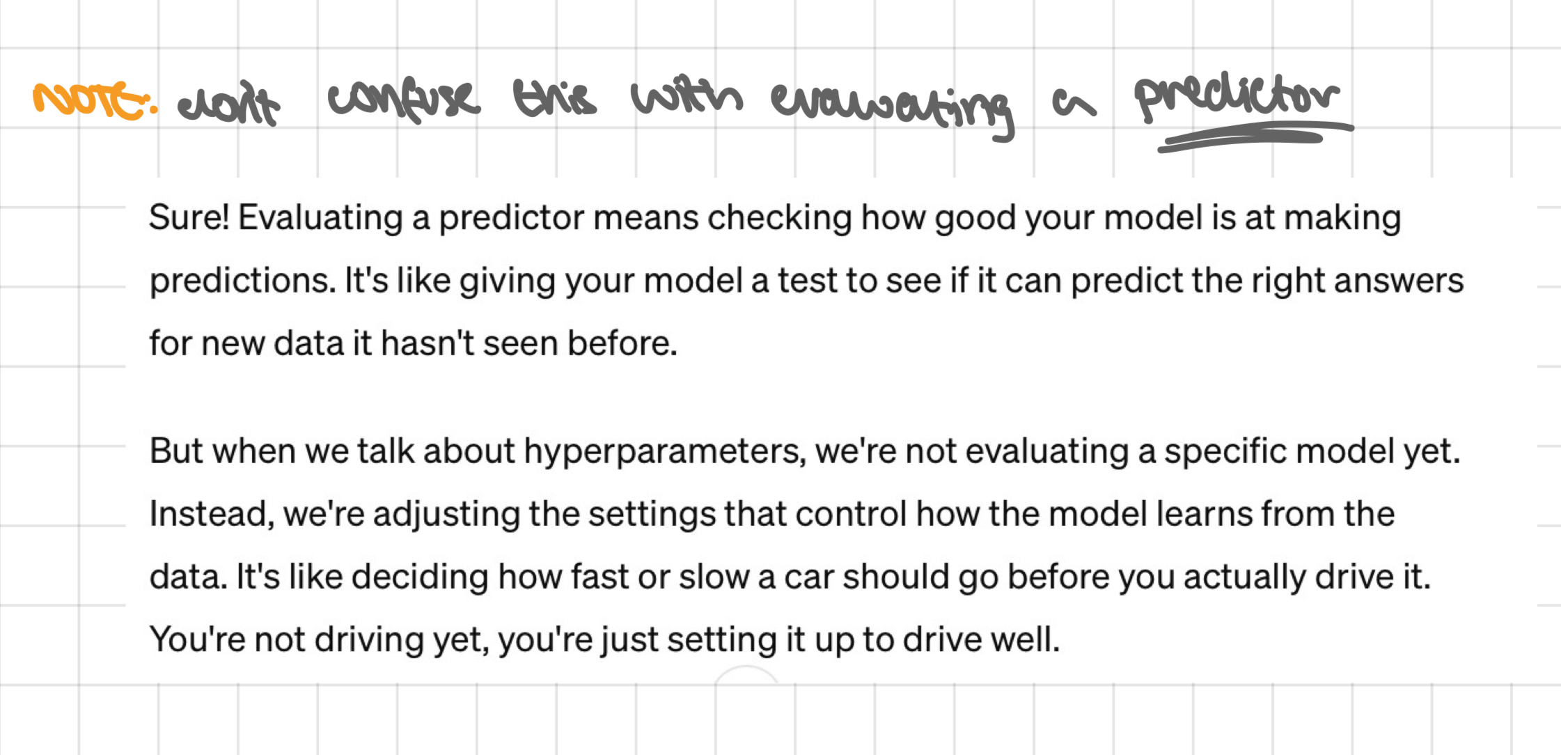
evaluation of a predictor before deployment

→ getting a predictor : first, train a model using data that’s already been annotated = teaching the model to make predictions based on examples we’ve given it

→ evaluation of a predictor serves it to estimate its future performance, before deploying it in the real world

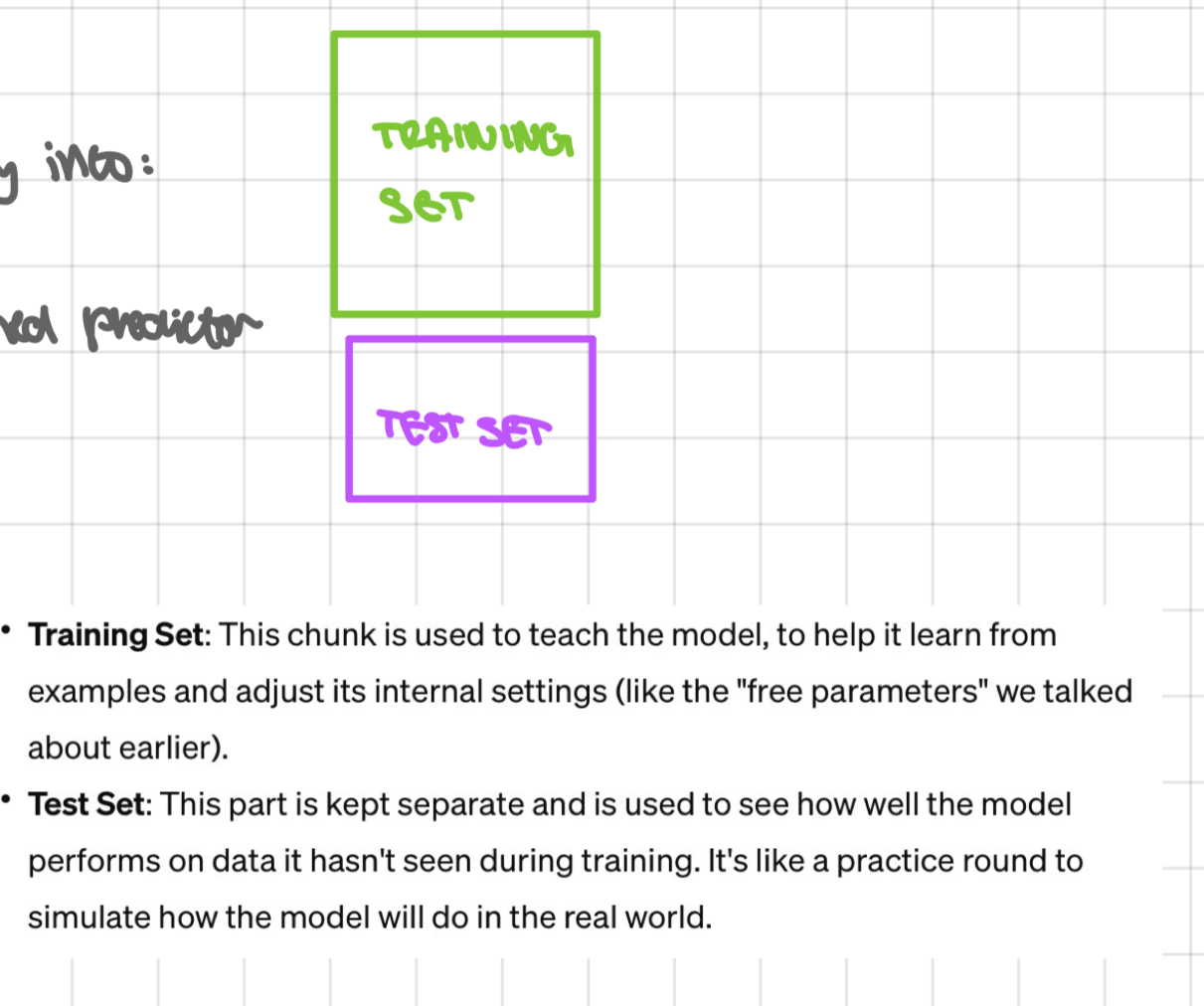
• to do so, always split available annotated data randomly into:

  • a training set - used to estimate the free parameters

  • a test set - used to evaluate the performance of the trained predictor before deploying it

  by doing this, = can have ↑ confidence our model will work well when we actually deploy it irl situations

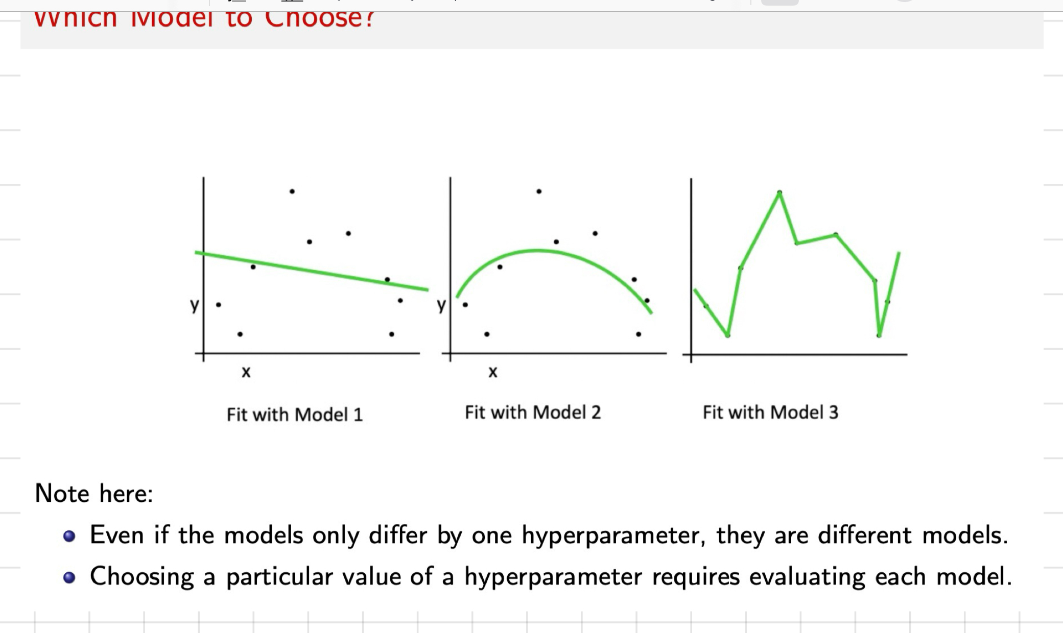
which model + how to set hyper parameters ?

• each hyper parameter value you choose creates a diff version of the model → e.g. changing the depth or width of a neural network creates a diff model

we need methods that evaluate each model

• for this evaluation, x use the cost function computed on the training data set, why?

  • the more complex (flexible) the model = the ✓ it’ll fit the training data

  • but, goal = predict well on future data

  • a model that has capacity to fit any training data will overfit

sets

training set = annotated data used for training within a chosen model

test set = annotated data used for evaluating the trained predictor before deploying it

none of these can be used to choose the model

• if you use the test set = x longer have an independent data set to evaluate final predictor before deployment

note: x confuse choosing hyper parameter w evaluating a predictor

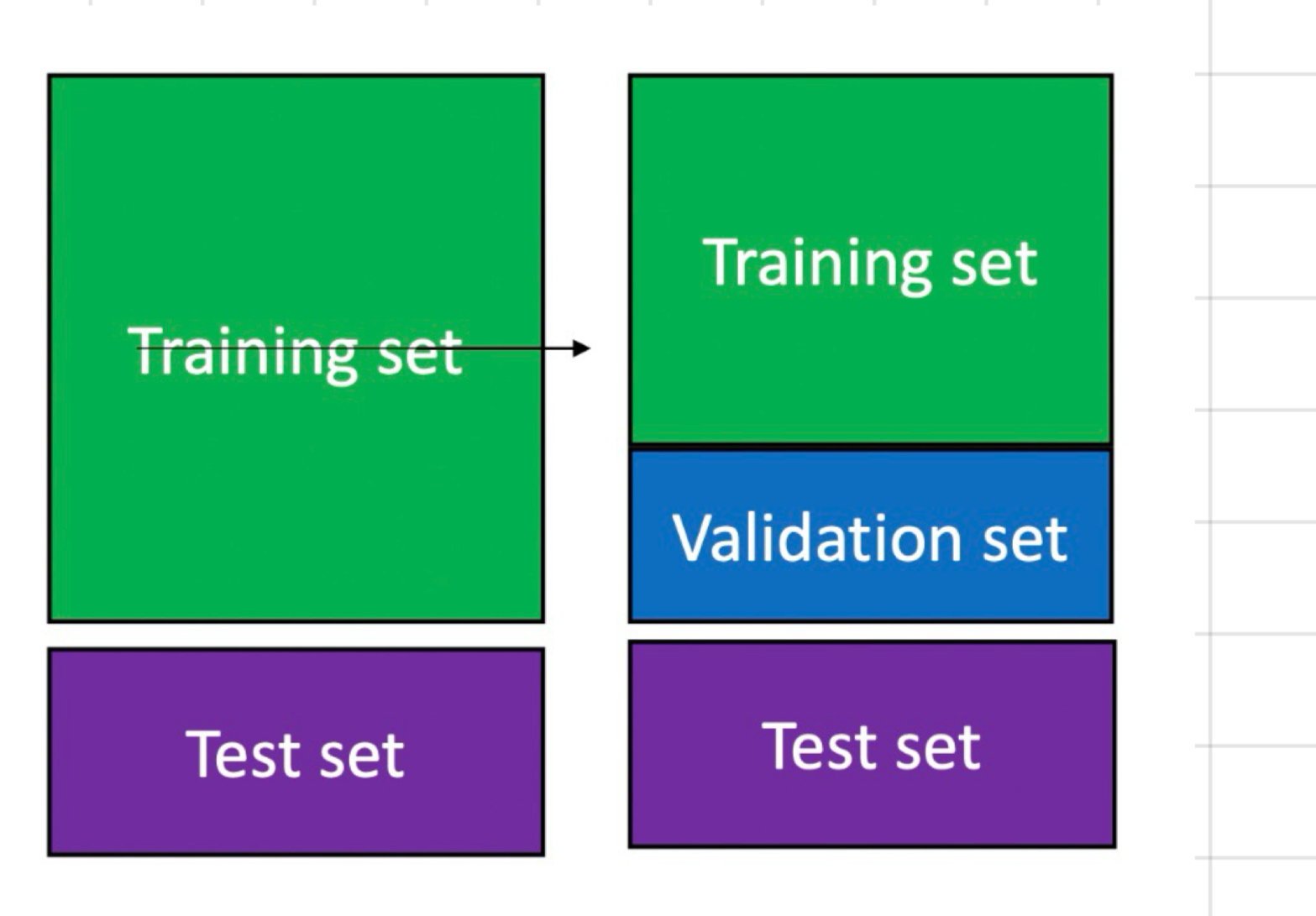
evaluating models for model choice

idea: choose between models or hyper parameters, separate a subset from training set to create a validation set

methods:

• hold out validation

• cross validation

• leave-one-out validation

method 1: hold out validation

steps:

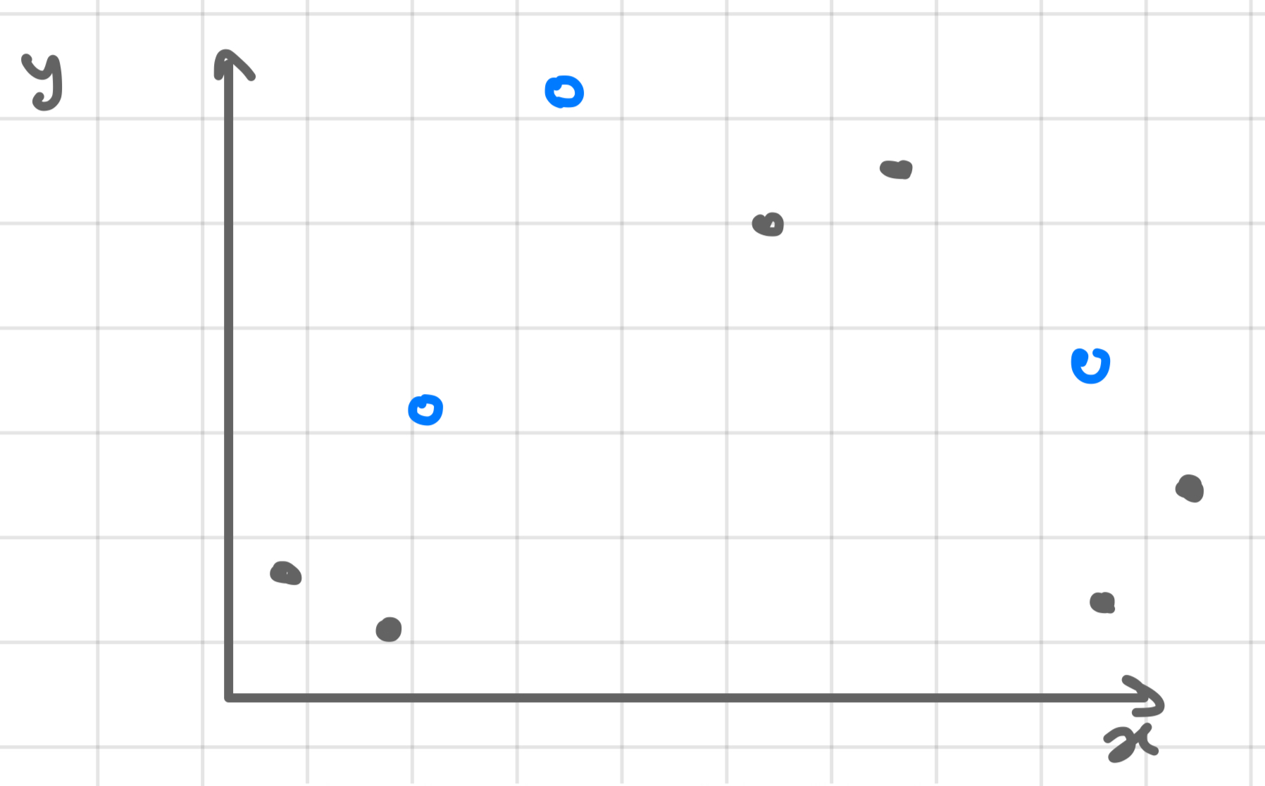
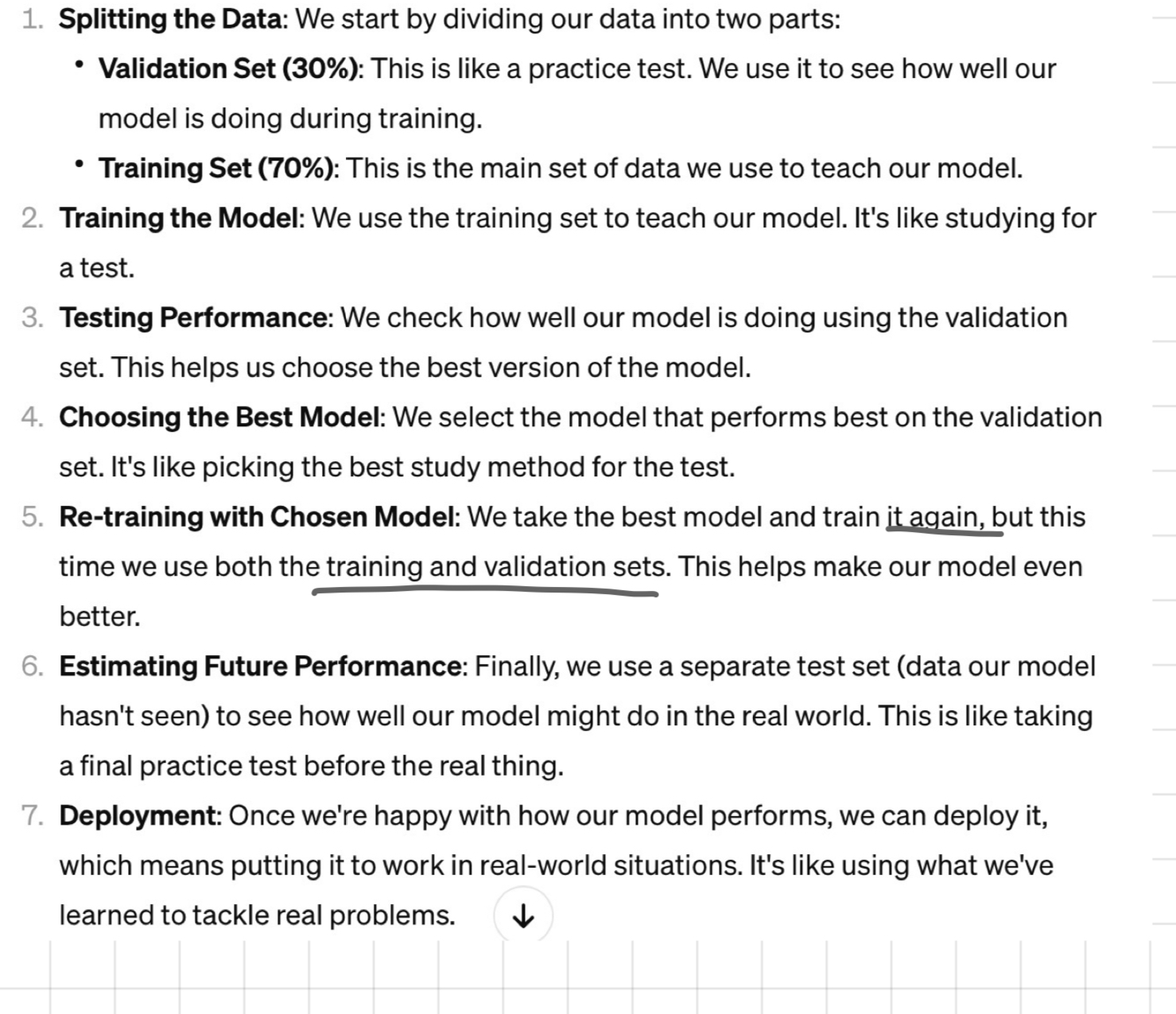
1. randomly choose 30% of data to form a validation set (blue data points)

2. remaining data forms the training set (black data points)

3. train your model on the training set

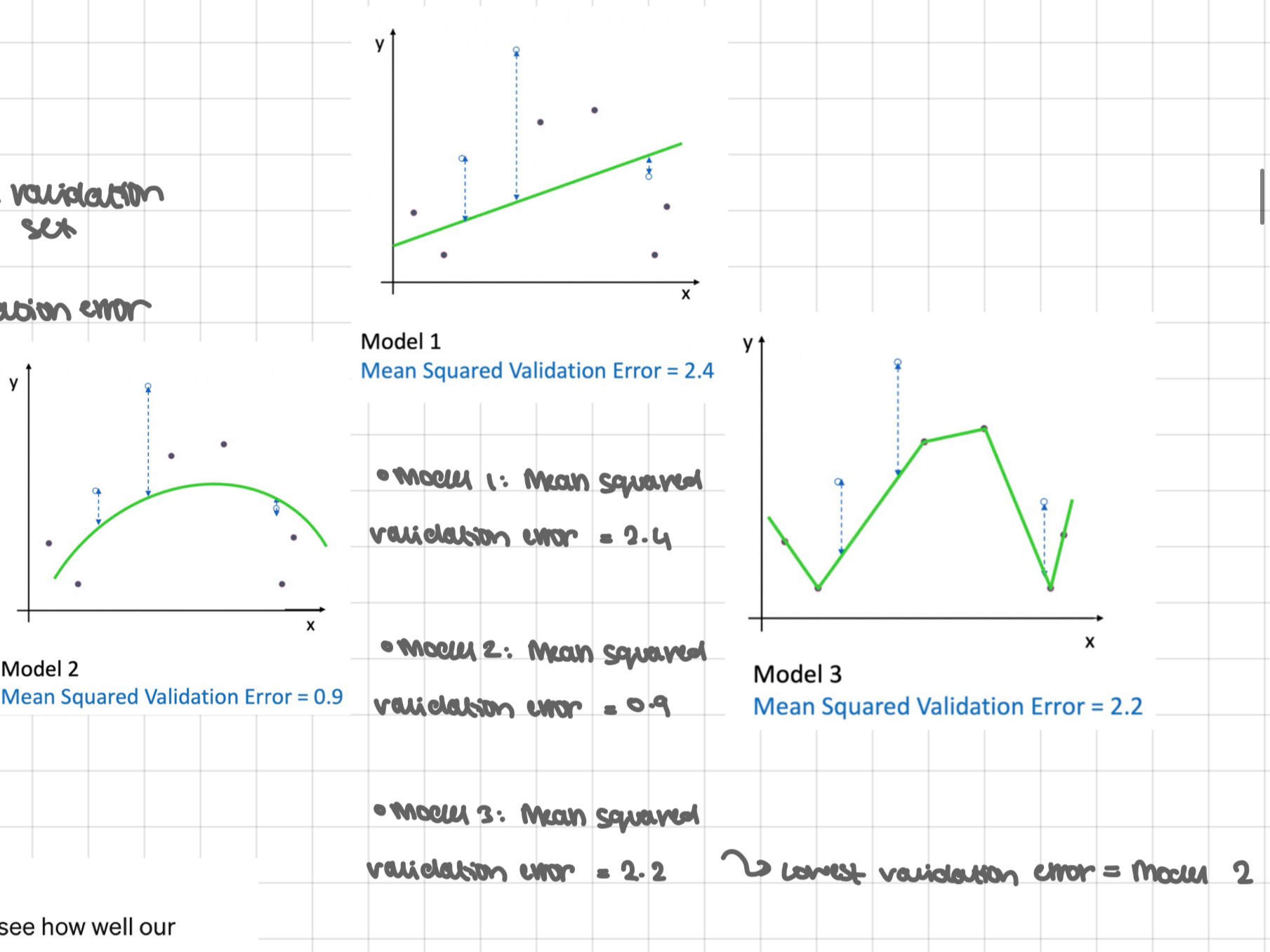
4. estimate the test performance in the validation set

5. choose the model with the lowest validation error

6. retrain the chosen model on joined training + validation to obtain predictor

7. estimate future performance of obtained predictor on test set

8. ready to deploy the predictor

continued

note on step 4: in practice, done differently in regression + classification

→ regression: compute the cost function (MSE) on the examples of the validation set (instead of the training set)

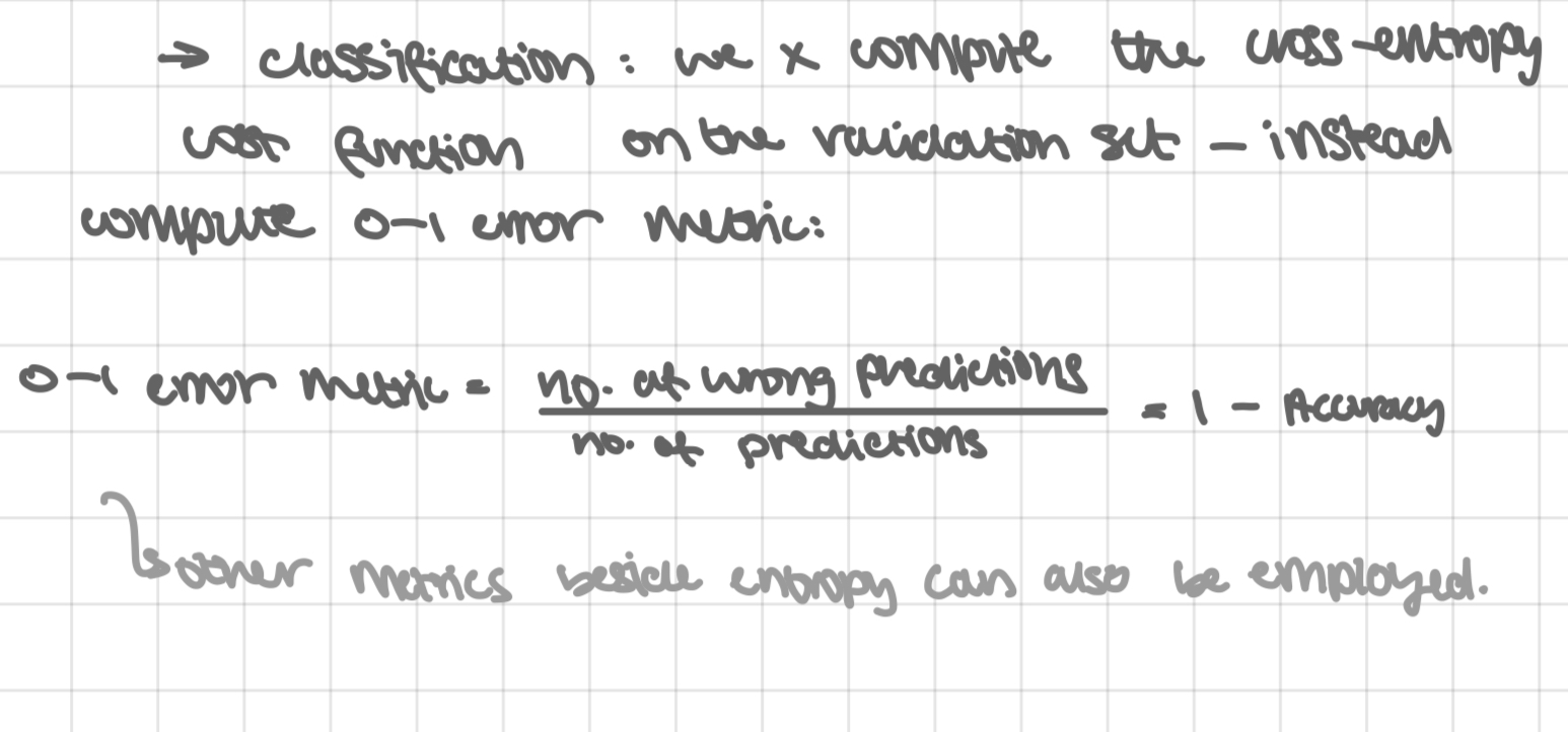
→ classification: we x compute the cross-entropy cost function of the validation set - instead compare 0-1 error metric:

0-1 error metric = no, of wrong predictions/no. of predictions = 1- accuracy

• other metrics beside entropy can also be employed

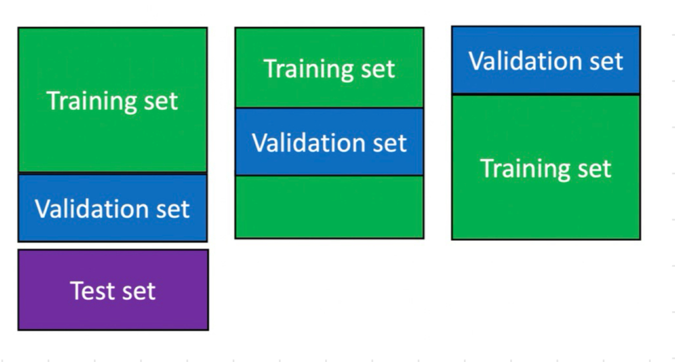
method 2: k-fold cross-validation

1. split the training set randomly into k (equal sized) disjoint sets (in this example, k=3)

2. use k-1 of those together for training

3. use the remaining one for validation

4. permute the k sets and repeat k times (rearrange w/o removing any elements)

5. average the performances of k validation sets

explanation of method 2 steps

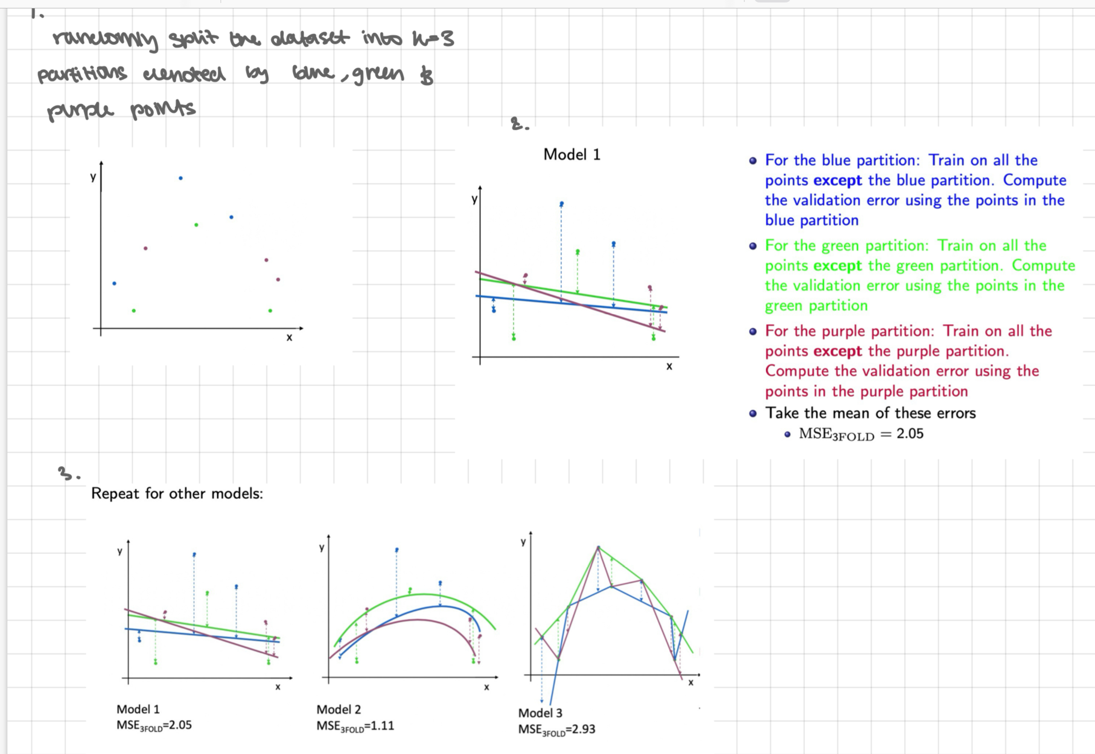
1. randomly split the dataset into k=3 partitions denoted by the blue, green + purple points

2. for the blue partition: train on all points except the blue partition. compute the validation error using the points in the blue partition. for the green partition: train on all points except the green partition. compute the validation error using the points in the green partition. for the purple partition: train on all points except the purple partition. compute the validation error using the points in the purple partition. - take the mean of these errors

3. repeat for the other models

   choose the model with the smallest avg 3-fold cross validation error - here in model 2

   • retrain with the chosen model on joined training + validation to obtain the predictor

   • estimate future performance of the obtained predictor on test set

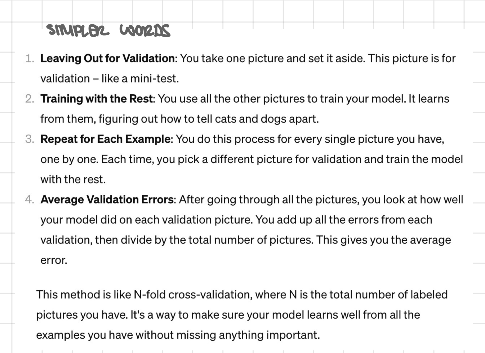
method 3: leave-one-out validation

1. leave out a single example for validation + train on all the rest of the annotated data

2. for a total of N examples, we repeat this N times, each time leaving out a single example

3. take the average of the validation errors as measured on the left-out points

4. same as n fold cross-validation where N is the no. of labelled points

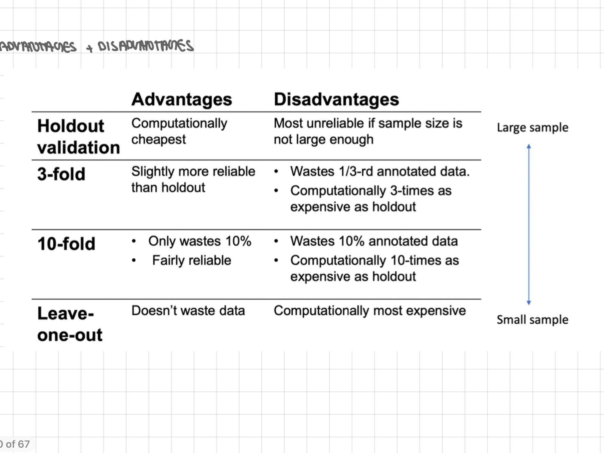
advantages + disadvantages of the methods