8.1: Distribution of the Sample Mean

Learning Objectives: (1. Describe the distribution of the sample mean: normal population 2. Describe the distribution of the sample mean: non-normal population)

RECALL that when studying things, we always have a ______________ of interest

Population

What do we want to know about the population of interest?

Certain characteristics, or (in stats language), Parameters

In practice, what is one key feature about parameters?

They are NEVER KNOWN

Since Parameters are never known, the best researchers can do is estimate. Describe this research process:

1. Define your population (what is your population? Make sure you have it.)

2. Take a sample of the population.

   • We want this sample to be representative and so our best easiest method to do this is to make the sample random.

3. Then we calculate a statistic.

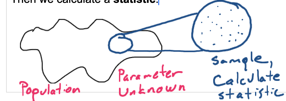
We would like to use our statistic as an estimate for the parameter, but we should ask ourselves a few guiding questions first.

• We’re not ready to answer these questions yet, but the remainder of the course is about answering these questions.

• Will the statistic and the parameter have equal values? (probably not)

• How close is our statistic to the parameter? In other words, how good is our estimate? (Who knows? No way telling)

• If we took a different sample, would we get the same statistic as in the first sample? (Probably not)

  • If not, how do we know which statistic is closer to the parameter? (We don’t!)

• If we don’t know our parameter’s value, how would we know how good of an estimate any statistic actually is? (We wouldn’t)

EXAMPLE: Let’s look at our data for mothers’ age at our births. 

Directions:

• To simplify our studies for now, we’ll restrict our current discussion to the mean.

  • For this example, treat the survey respondents as the population, even though normally, survey respondents are a sample. Once we do that, we’ll take samples from that population to study the relation between sample and the population.

Population-Level Data for Mother’s Age at Your Birth (note we will treat our class as the “entire population”)

1. Identify the Population Mean

   = 29.27

2. Take six samples of size n = 5

• Sample 1 = { 28, 35, 34, 30, 39}, Mean₁ = 33.2

• Sample 2 = { 26, 29, 30, 22, 36}, Mean₂ = 28.6

• Sample 3 = {33, 22, 30, 40, 35}, Mean₃ = 32

• Sample 4 = { 27, 30,20, 25, 30 }, Mean₄ = 26.4

• Sample 5 = { 28, 27, 30, 32, 30 }, Mean₅ = 29.4

• Sample 6 = { 25, 19, 30, 35, 28 }, Mean₆ = 27.4

Why are statistics such as x-bar random variables?

• Because their value varies from sample to sample.

• Because they have probability distributions associated with them.

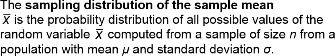
What is a sampling distribution of a statistic?

• probability distribution for all possible values of the statistic computed from a sample of size n.

Distribution of the Sample Mean: How to illustrate Sampling Distributions

1. Step 1: Obtain a simple random sample of size n.

2. Step 2: Compute the sample mean.

3. Step 3: Repeat steps 1 and 2 until all distinct simple random samples of size n have been obtained.

**(Remember, in reality, we’ll never really have access to the entire population, so this process isn’t really a thing – this is a theoretical exercise to help us understand better)

Goal Check:

Understand…

• that we have/know a population.

• how we sample from that population.

• how we compute the mean of that sample.

• that we do that again and again.

• that we collect those means and try to get a feel for that collection.

Summary:

• -The shape of the sampling distribution gets increasingly “normalish” the larger the size of the sample. This has a special name we’ll learn later.

• -If the population itself is normal, the sampling distribution will also be normal, regardless of sample size.

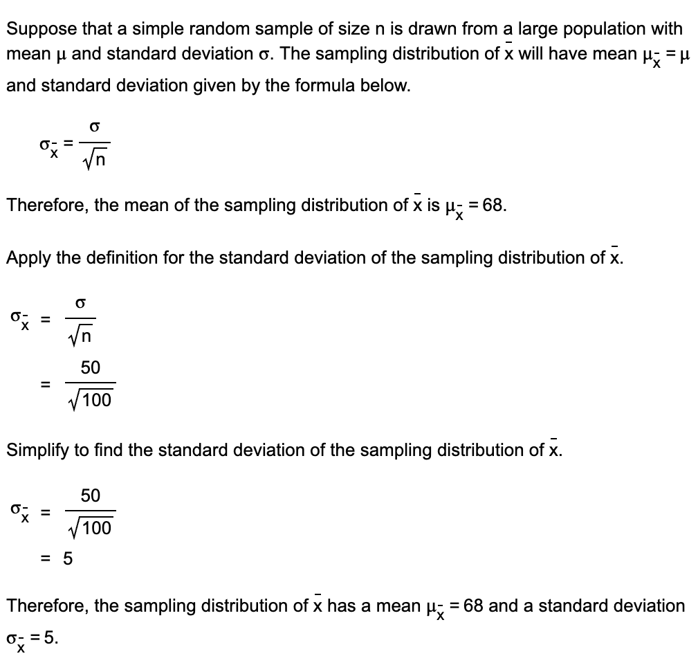
• -The mean of the sampling distribution equals the population mean.

• -The standard deviation of the sampling distribution is smaller than the standard deviation of the population.

• -The standard deviation of the sampling distribution decreases as we increase the sample size with which we create our population distribution.

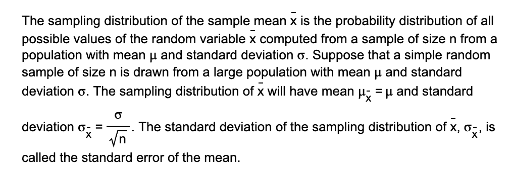
The Mean and Standard Deviation of the Sampling Distribution of X-Bar

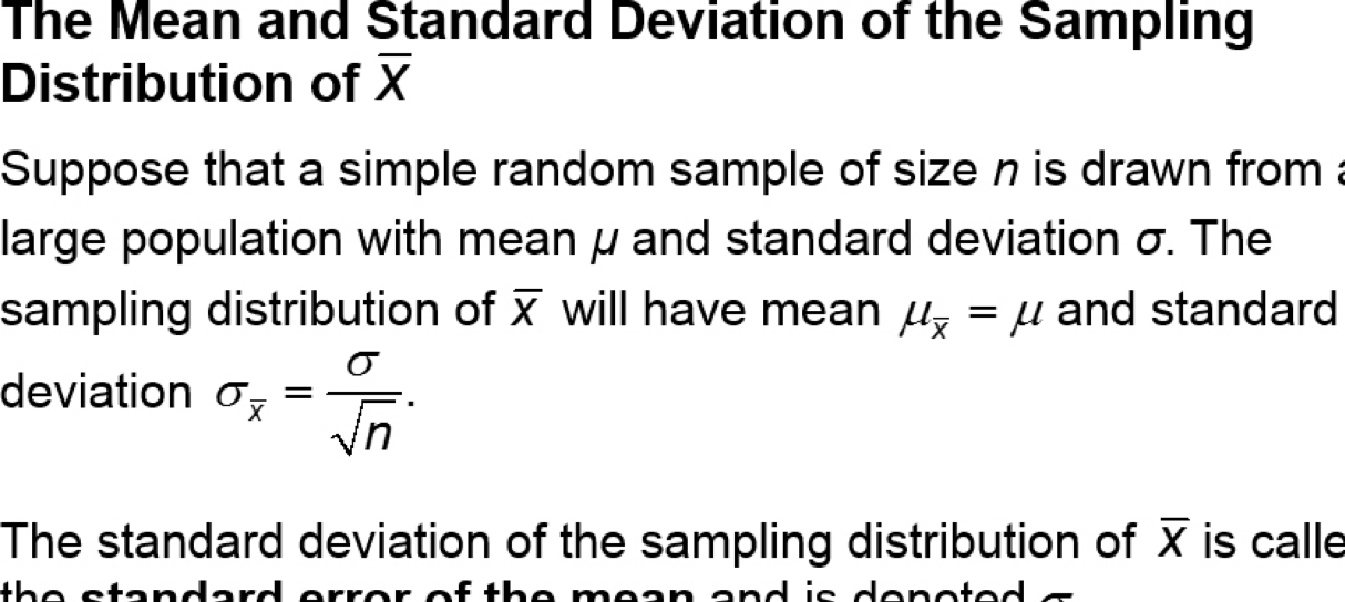
The standard deviation of the sampling distribution of x̄ (denoted σ_x̄ ) is called the​ _____ _____ of the​ _____

STANDARD ERROR of the MEAN

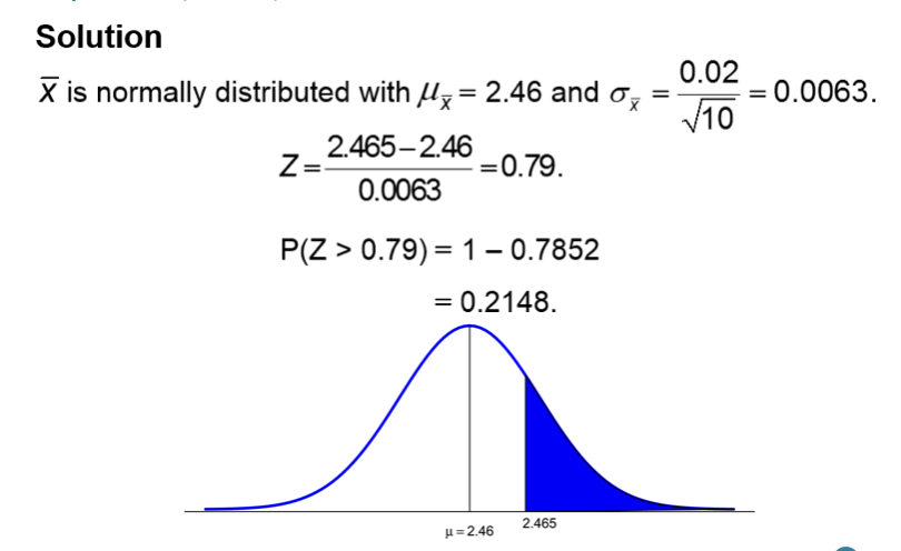
Example: Describing the Distribution of the Sample Mean

The weights of pennies minted after 1982 are approximately normally distributed with mean 2.46 grams and standard deviation 0.02 grams. What is the probability that in a simple random sample of 10 pennies minted after 1982, we obtain a sample mean of at least 2.465 grams?

Central Limit Theorem

States that regardless of the shape of the underlying population, the sampling distribution of x̄ becomes approximately normal as the sample size (n) increases.

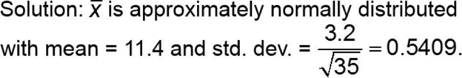
Example 2: Using the Central Limit Theorem

Suppose that the mean time for an oil change at a “10-minute oil change joint” is 11.4 minutes with a standard deviation of 3.2 minutes.

a) If a random sample of n = 35 oil changes is selected, describe the sampling distribution of the sample mean.

b) If a random sample of n = 35 oil changes is selected, what is the probability the mean oil change time is less than 11 minutes?

a) ANSWER in pic

b) If a random sample of n = 35 oil changes is selected, what is the probability the mean oil change time is less than 11 minutes?

b) ANSWER in pic

Suppose a simple random sample of size n is drawn from a large population with mean μ_x=_____ and standard deviation σ_{x^{= ________}}

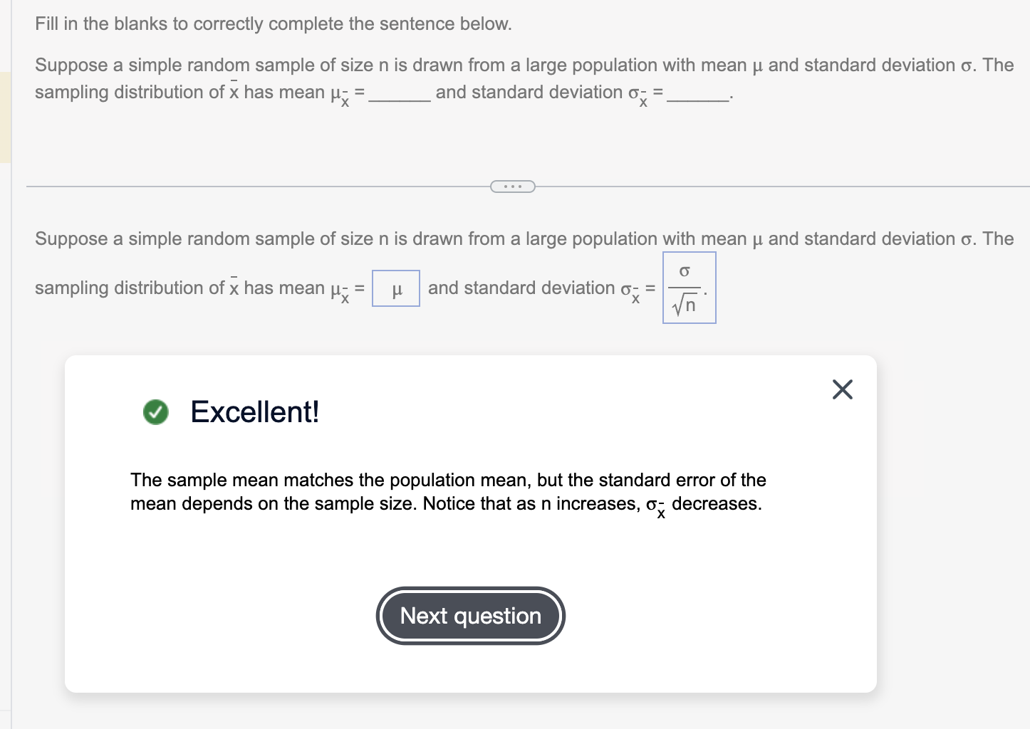
The sampling distribution of x-bar for simple random samples of size n has the same mean as the population.

• M_x-bar = 81

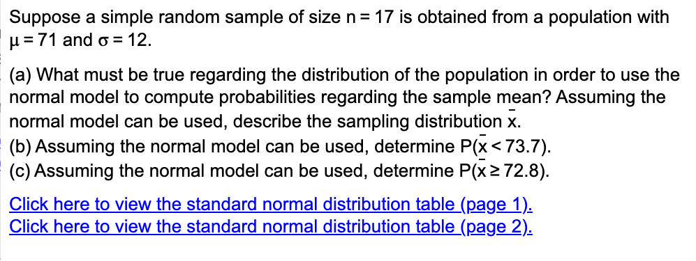
Remember: The sample size must be greater than or equal to 30 or the population must be normally distributed in order to use the normal model to compute probabilities regarding the sample mean.

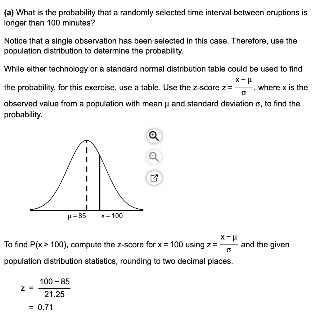
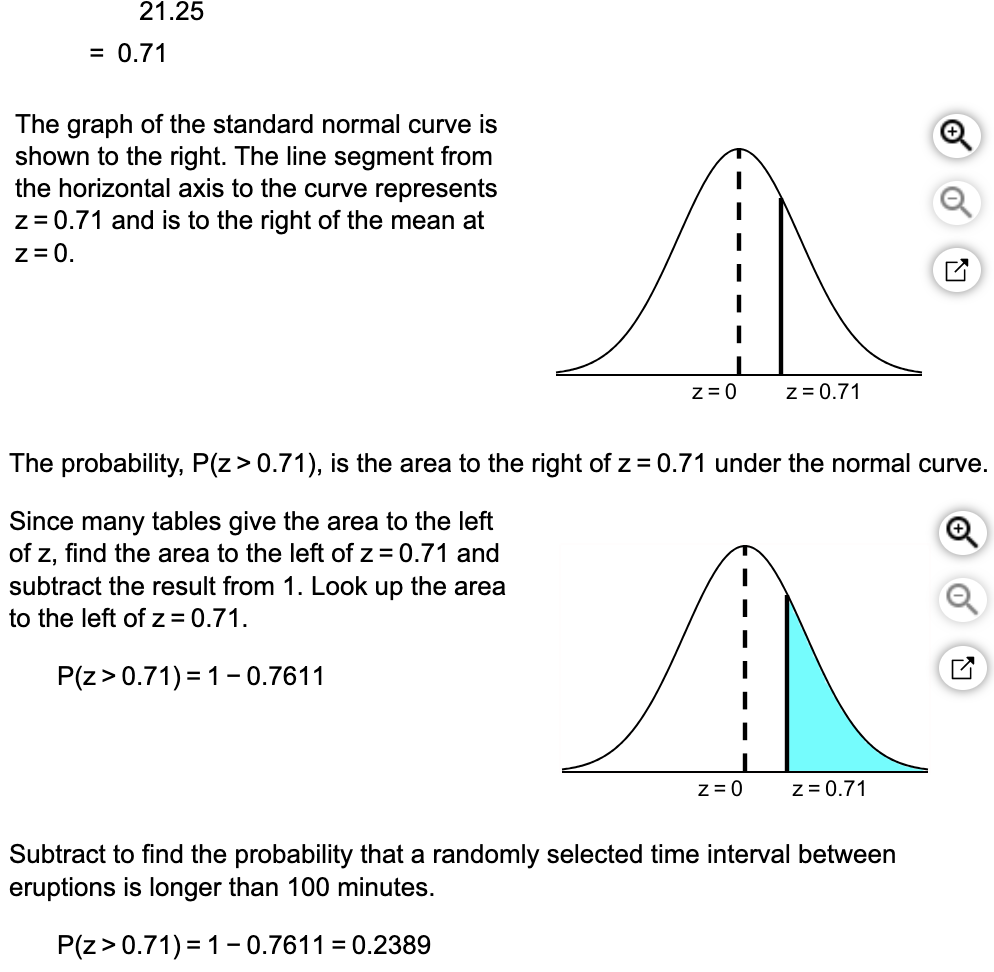
​(a) What is the probability that a randomly selected time interval between eruptions is longer than 100 minutes?

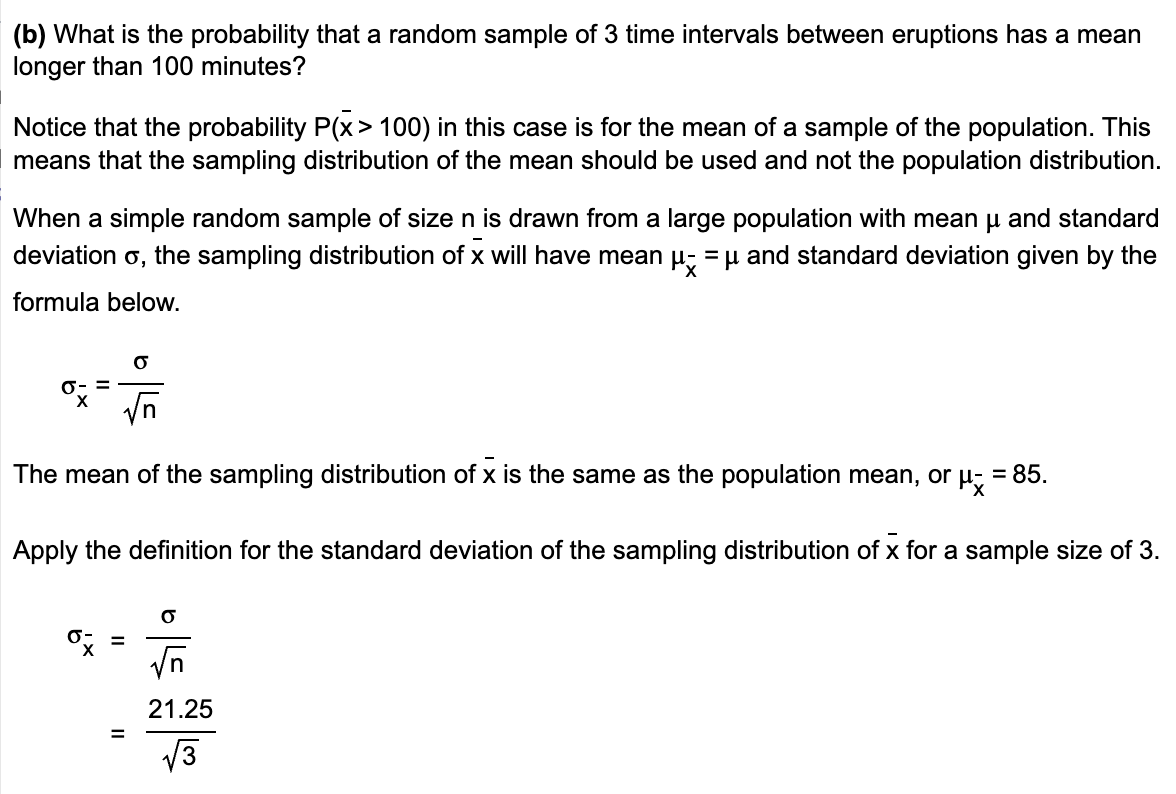
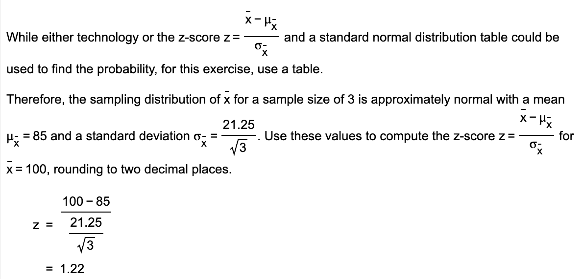
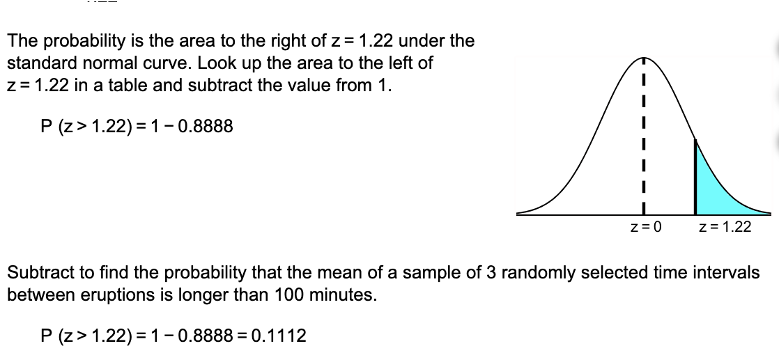
​(b) What is the probability that a random sample of 3 time intervals between eruptions has a mean longer than 100 minutes?

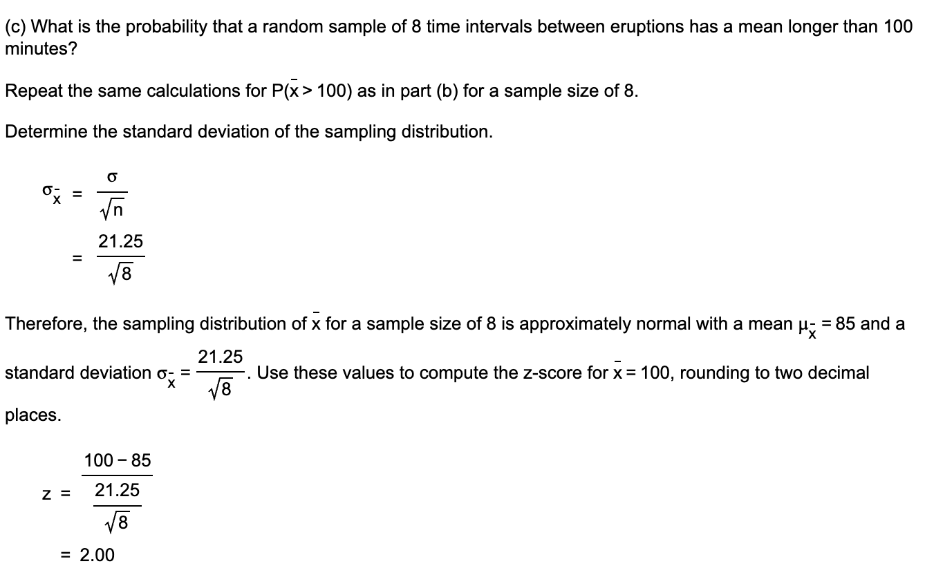
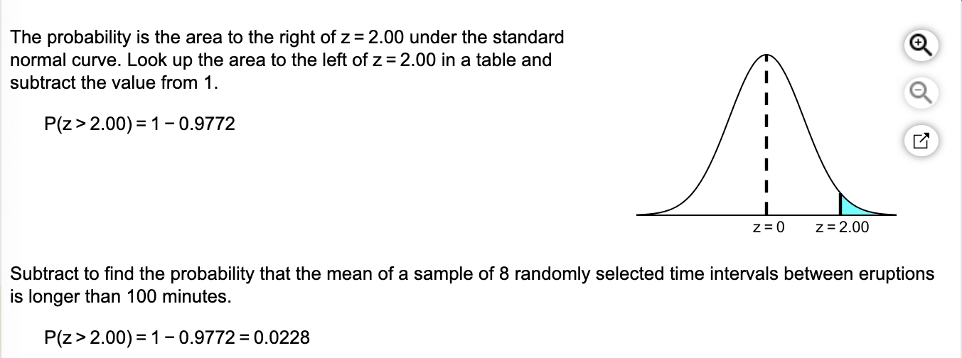
​(c) What is the probability that a random sample of 8 time intervals between eruptions has a mean longer than 100 minutes?

​(d) What effect does increasing the sample size have on the​ probability? Provide an explanation for this result.

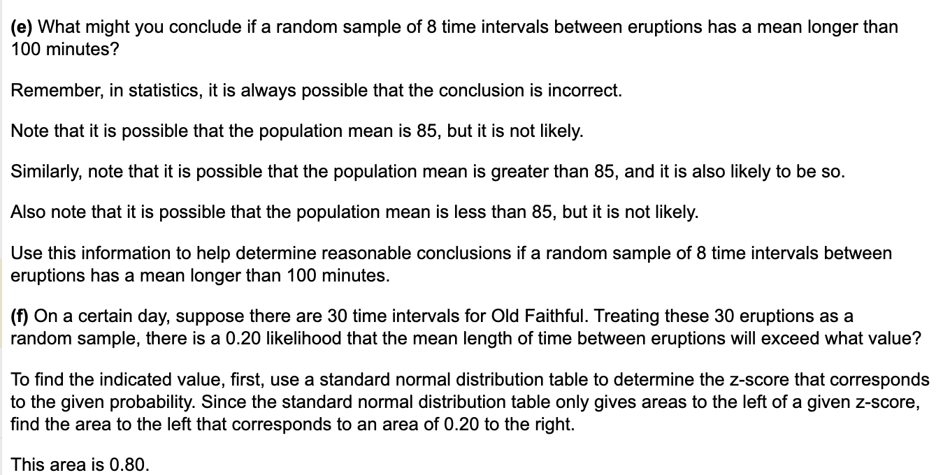
​(e) What might you conclude if a random sample of 8 time intervals between eruptions has a mean longer than 100 minutes?

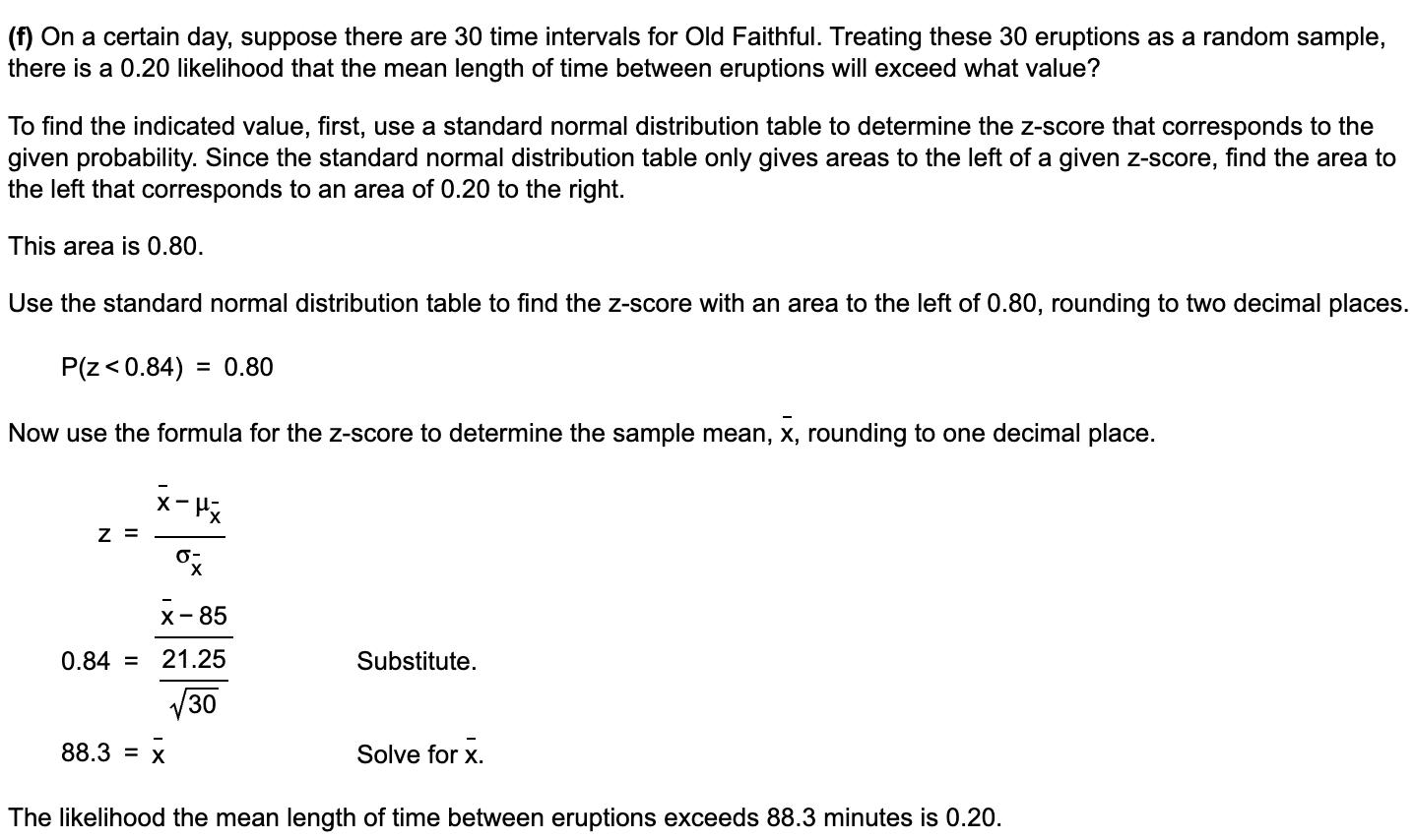
​(f) On a certain​ day, suppose there are 30 time intervals for Old Faithful. Treating these 30 eruptions as a random​ sample, there is a 0.20 likelihood that the mean length of time between eruptions will exceed what​ value?

---

---

---

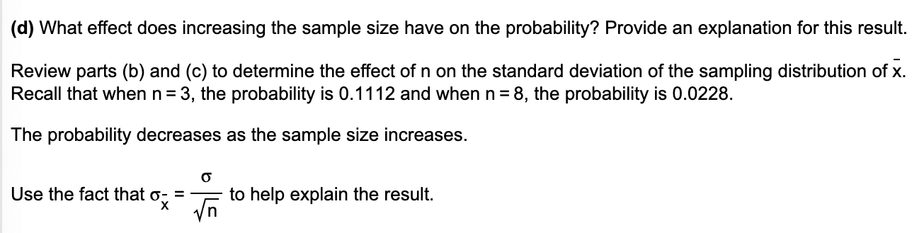
And if the sample size​ increases, the probability decreases because the variability in the sample mean increases

---

---

A simple random sample of size n = 47 is obtained from a population that is skewed left with μ = 84 and σ = 9. Does the population need to be normally distributed for the sampling distribution of x-bar to be approximately normally​ distributed? Why? What is the sampling distribution of x-bar?

No. The central limit theorem states that regardless of the shape of the underlying​ population, the sampling distribution of x-bar becomes approximately normal as the sample​ size, n, increases.

The sampling distribution of x-bar is: μ_x= 84 and σ_x = 1.313