Macro Topic B1 - The medium run (AD-AS model)

Assumptions (Price and Labour)

Sticky prices - Price expectations fixed in SR but can change in MR

No inflation in equilibrium (only in SR)

Labour force fixed but uneployment (u) can vary

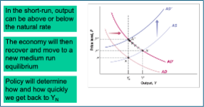
Medium run model

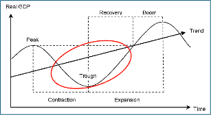
The economy recovers naturally, the policy just speeds it up

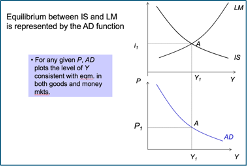
Aggregate Demand (AD)

shows combinations where goods & money market are in equilibrium

Aggregate Supply (AS)

shows when labour market is in equilibrium

Employment rate

(N/L) = share of the labour force employed

Unemployment rate

u = (L-N) / L

reservation wage

• The wage that would make them indifferent between working or being unemployed

unique to everyone

What does the bargaining power of L depend on

the nature of the job and skills required (skills vs. unskilled workers)

labour market conditions - Workers can demand a higher wage if there is less unemployment

Efficiency wage theory

There is a link between productivity / efficiency of workers & wage they are paid

Wage determination from perspective of firms

To be useful to an employer a worker has to exert effort on the job

o When the employer hires a worker at an hourly wage or annual salary they cant determine the level of effort that they will actually do

 In the presence of this imperfect / asymmetric information employers design contracts that minimise its effects

• Paying a wage in excess of the reservation wage creates a cost from losing their job and ensures effort by the worker

• Firms may want to pay wages higher than the reservation wage to encourage workers’ productivity and reduce turnover costs

o Hiring + training + firing costs

Wage determination from perspective of labour:

• To produce output firms need labour.

• Output varies over the business cycle

• To induce more workers to provide labour the real wage must rise.

• Wages therefore depend on the point in the business cycle.

What affects W

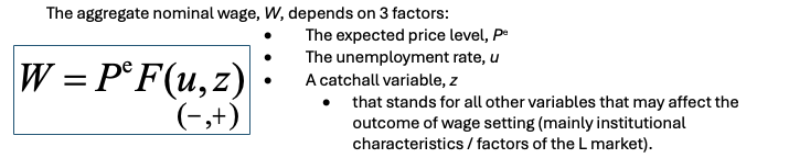
expected price level (P^e)

Both workers and firms care about real wages (W/P) , not nominal wages (W)

·      Workers want to know how many goods they can actually buy with their wages

·      Firms care about the wage they pay relative to the price of the goods they sell

Why P^e not P

·      Work contracts set the nominal wage for a given duration (usually, 2-3 years).

o   Wage contracts cause price stickiness

·      When workers sign their contracts they make predictions about the future price level.

o   work-hours supplied depends on the expected real wage, W/P^E

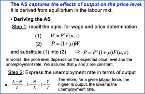
P^E ↑  →  W ↑

Unemployment rate (u)

u ↓ → W ↑

Higher unemployment weakens workers’ bargaining power, forcing them to accept lower w

o (pushes them closer to their reservation wage – and so more willing to be unemployed).

Higher unemployment strengthens bargaining of firms allowing then to pay lower wages and still keep workers willing to work

o (consistent with efficiency wage hypothesis).

Bargaining power over the business cycle

NOT CONSTANT

In recession L has less bargaining power than firms and so get a lower w

In boom L has more bargaining power so w is higher

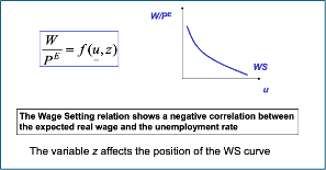
Other factor variable (z)

z ↑ → W ↑

Includes: unemployment benefits + minimum wage + job protection laws and regulations

Price determination

Prices set by firms depend on costs. Costs depend on:

o The technology of production

 the function linking inputs and produced output – how much labour they need to produce a given level of output

o Input prices

 Wages only as L only input

Y = AN

N is labour input & A is productivity

 We set A = 1 so Y=N

 Unit cost of production = W

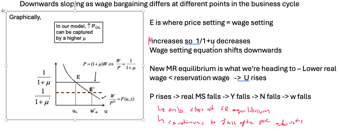
Price setting

Under imperfect competition, firms set P as a mark-up over MC

o   P = (1+x)W

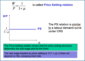
o   W/P = 1/1+x   x is a measure of the market power of firms

Under Perfect comp markup = 0

o   P=MC → Workers paid their marginal product

 

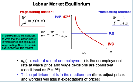
Price setting determines the real wage paid by firms (W/P doesnt depend on u)

L market equilibrium

Wage setting changes at different partd of business cycle

What if u falls?

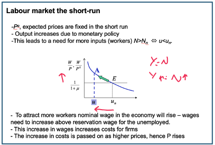
We assume in SR PE are fixed

W rises as the relative bargaining power of L rises

Real wages rise above equilibrium (W/P > W/ PE) → A

This leads to a rise in P (P > PE)

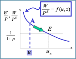
SR ends and MR begins when workers can renegotiate contracts – update PE (P>PE) → Output will fall as expectations updated

This gives bargaining power back to firm until we rereach the equilibrium

PE↑ and so for a given nominal W, => N↓ (u↑ ) until ΔW= ΔP= ΔPE , and the economy is back at point E where wage setting and price setting decisions are consistent with each other (u=un).

What if market power (x) increases?

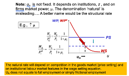
Natural rate of unemployment depends on z & x

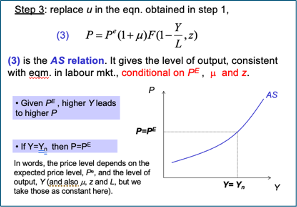
Deriving AS

AS properties

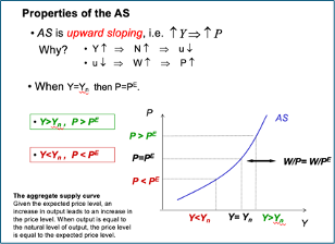
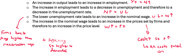
An increase in output leads to an increase in the price level (move along AS) → In SR we move along AS as Pe are fixed

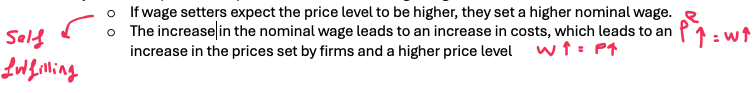
An increase in the expected price level leads, one-for-one, to an increase in the actual price level (shift AS)

AS is upward sloping

Why an increase in output leads to an increase in the price level (AS curve)

Why an increase in the expected price level leads, one-for-one, to an increase in the actual price level

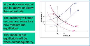
AS and MR equilibrium

AD - P & Y

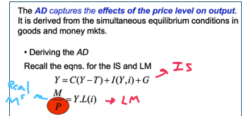
How is AD affected when P rises

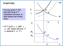
AD shifts

AD shifts either from change in MS or by a change in fiscal variables (G or T)

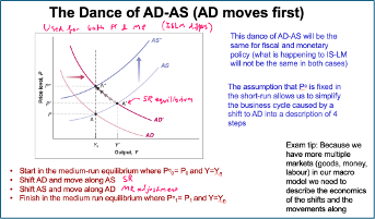
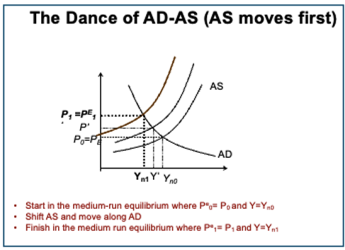
Dance of AD & AS (Demand side shock)

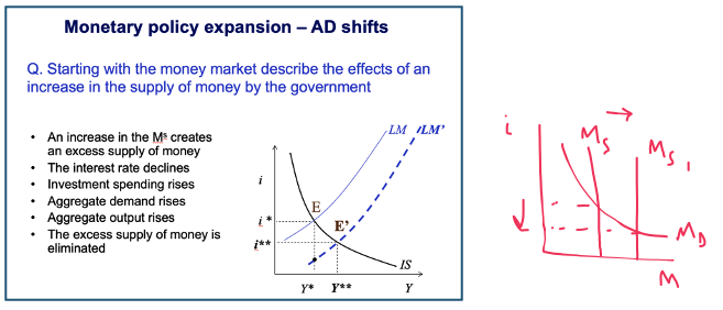
Expansionary MP

Expansionary MP effects on L market in SR

Expansionary MP effects on SR equilibrium

Adjustment back to MR after expansionary MP (AD/AS)

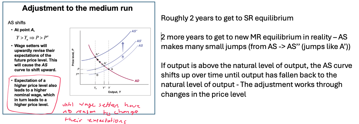
AS shifts upwards in many little jumps until back at MR equilibrium (Y_n)

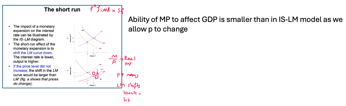
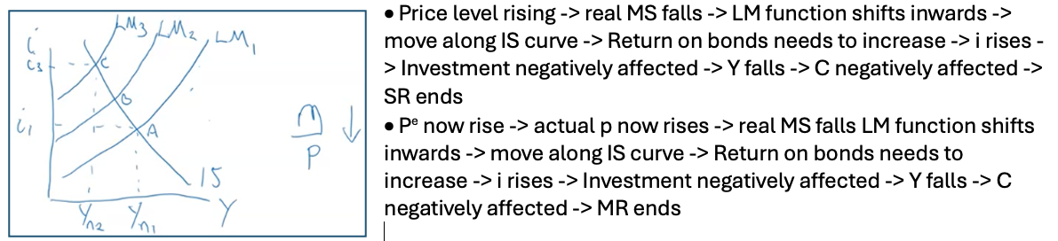
Adjustment back to MR after expansionary MP (IS-LM)

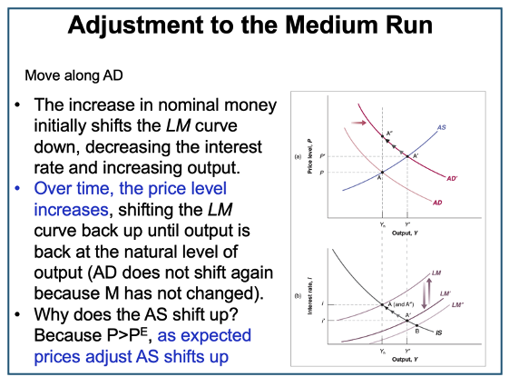
LM shifts back slowly to MR equilibrium as p increases - this is shown by movement along AD

p adjusts BUT i is constant

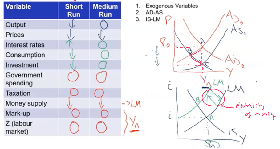
Neutrality of money

If MS up 10% then price level up 10% as well

A change in MP doesn’t affect any of the real variables in the model (GDP, C & I) as Income and i unchanged

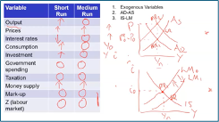
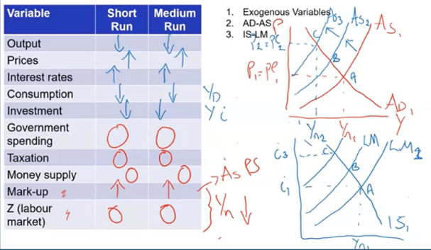
•       SR - MP expansion leads to an increase in Y, a decrease in i and an increase in p

•       In MR, the increase in nominal money is reflected entirely in a proportional increase in the price level. The increase in nominal money has no effect on output or on the interest rate.

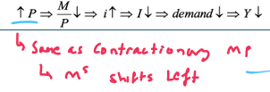
Contractionary MP

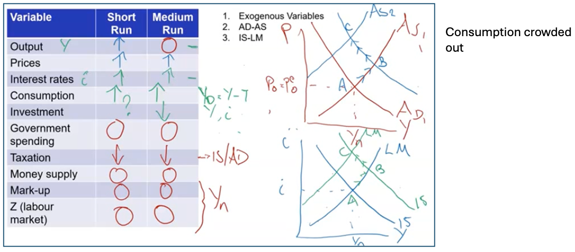
Contractionary FP (G down) overall

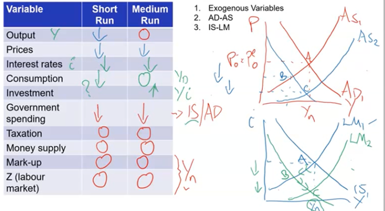
With FP change we shift IS first then we move LM (unlike MP where LM shifts out then shifts back in MR equilibrium)

The composition of Y has changed (I ^ but G down)

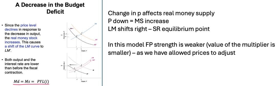
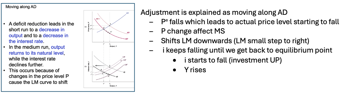
Contractionary FP explained

Decrease in G → fall in Y → IS shifts inwards

Y falls → M^d falls → excess M^s decreases i → I rises so effect ambiguous

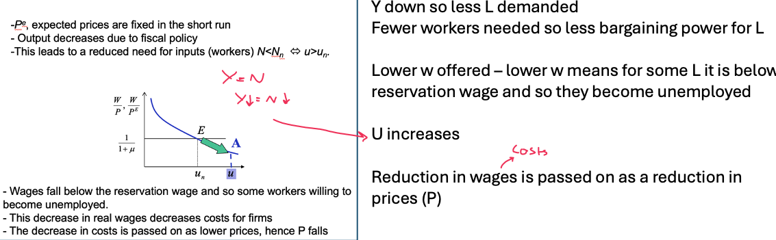
Contractionary FP effect on L market in SR

Con

Contractionary FP SR (IS-LM)

C

Contractionary FP MR (L market)

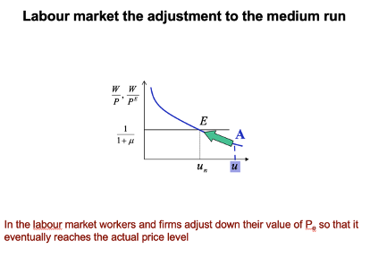
P^e adjusts & Y starts to rise again 

Relative bargaining power shifts back to workers (over firms)

Firms willing to offer higher w again

More people employed as Higher W > reservation wage → U falls

Contractionary FP MR (AD/AS)

Budget defecit effects

In SR it decreases Y + may decrease I

In MR Y returns to Y_n + i falls → I ^

Our conclusions would be modified if we take into account the effects on capital accumulation - In the LR, the level of output depends on the capital stock in the economy

Multiplier values for different models

K cross → 4

OBR → 0.6

AD/AS in MR → 0

Expansionary FP (T down)

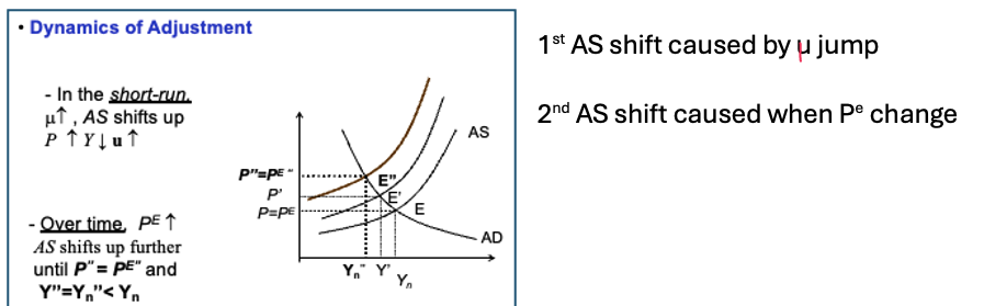
Dance of AD AS (Supply side shock)

With supply side shocks, AS shifts 2x

1^st shift – P^e held constant + moving along AD (talk about demand side)                                                         SR

2^nd shift – P^e shifts causing AS to shift        MR

Economy never recovers - Y_n + U_n + i + p all change in MR

Negative Supply side shock overall

If cost of production has shock (oil shock 1970 or Ukraine) then firs increase markup (x)

Negative Supply side shock L market

Negative Supply side shock explained (AD/AS)

Negative Supply side shock explained (IS-LM)

Limitations of AD-AS model

• Effects of policy depend on the slopes of IS and LM

• No inflation + no GDP growth in MR – not realistic

• Consumption depends only on current disposable income – simplistic

• Closed economy model – no interaction with RoW

• Results depend on the assumption of adaptive expectations in labour market