Econometrics

SW Figure 15.1b. Which of the following observation is true about the figure above?

a. There is no obvious trend in the growth rate of US GDP.

b. There is a persistent downward trend in the growth rate of US GDP.

c. The growth rate of US GDP shows strong weekly seasonality.

d. The growth rate of US GDP experienced a structural break in 1996.

There is no obvious trend in the growth rate of US GDP.

SW Figure 15.2c. Which of the following observation is true about the figure above on the log of Japan Index of Industrial Production (JIIP)?

a.     There is a persistent downward movement in the growth rate of the log of JIIP.

b.     There is no persistence in the log of JIIP.

c.     The log of JIIP experienced a structural break in 2000.

d.     The log of JIIP is stationary.

There is a persistent downward movement in the growth rate of the log of JIIP.

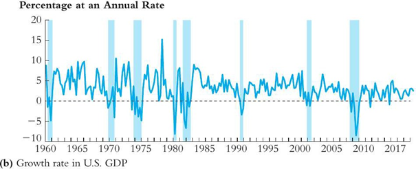
SW Figure 15.1b. Which of the following observation is true about the figure above?

a. There is no obvious trend in the growth rate of US GDP.

b. There is a persistent downward trend in the growth rate of US GDP.

c. The growth rate of US GDP shows strong weekly seasonality.

d. The growth rate of US GDP experienced a structural break in 1996.

There is no obvious trend in the growth rate of US GDP.

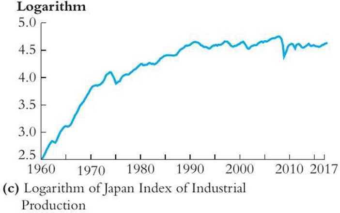
SW Figure 15.2c. Which of the following observation is true about the figure above on the log of Japan Index of Industrial Production (JIIP)?

a.     There is a persistent downward movement in the growth rate of the log of JIIP.

b.     There is no persistence in the log of JIIP.

c.     The log of JIIP experienced a structural break in 2000.

d.     The log of JIIP is stationary.

There is a persistent downward movement in the growth rate of the log of JIIP.

Certain conditions are needed in order to make reliable forecasts with time series data. Which of the following is not needed?

a.     The regression has high explanatory power.

b.     The coefficients have been estimated precisely.

c.     The presence of omitted variable bias.

d.     The regression is stable over time.

The presence of omitted variable bias.

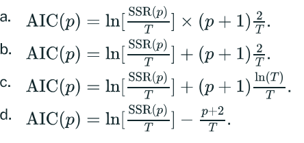
How is the Akaike Information Criterion (AIC) defined?

 

$AIC(p)=ln⁡[SSR(p)/T]+(p+1)2/T$ is a measure of model quality that balances goodness of fit and complexity.

What do we use the AIC statistic for?

a.     As an alternative to the BIC statistic when the sample size is small, say T < 50.

b.     To test for serial correlation.

c.     To help a researcher chose the number of lags in a time series with multiple predictors.

 

To help a researcher chose the number of lags in a time series with multiple predictors.

What is an autoregression?

a.     A regression model that relates a time series variable to its past values.

b.     A regression to predict sales in the auto industry.

c.     A regression that allows for the errors to be correlated.

d.     A regression of a dependent variable on lags of regressors.

 

A regression model that relates a time series variable to its past values.

What is the random walk model an example of?

a.     A deterministic trend model.

b.     A binomial model.

c.     A stationary model.

d.     A stochastic trend model.

A stochastic trend model.

What does stationarity mean?

a.     The time series has a unit root.

b.     The forecasts remain within 1.96 standard deviation outside the sample period.

c.     The error terms are not correlated.

d.     The probability distribution of the time series variable does not change over time.

The probability distribution of the time series variable does not change over time.

This means that the statistical properties such as mean and variance remain constant over time, allowing for reliable modeling and forecasting.

The formulae for the AIC and the BIC are different. Which is usually preferred?

a.     The difference is irrelevant in practice since both information criteria lead to the same conclusion.

b.     AIC is preferred because it is easier to calculate.

c.     BIC is preferred because it is a consistent estimator of the lag length.

BIC is preferred because it is a consistent estimator of the lag length.

Stochastic trends can cause problems for inference. Which one of the following is not a consequence of stochastic trends?

a.     The t-statistics on regression coefficients can have a nonnormal distribution, even in large samples.

b.     The model can no longer be estimated by OLS.

c.     The estimator of an AR(l) is biased towards zero if it's true value is one.

d.     The presence of spurious regression.

The model can no longer be estimated by OLS.

The ADL(p, q) model is represented by the following equation

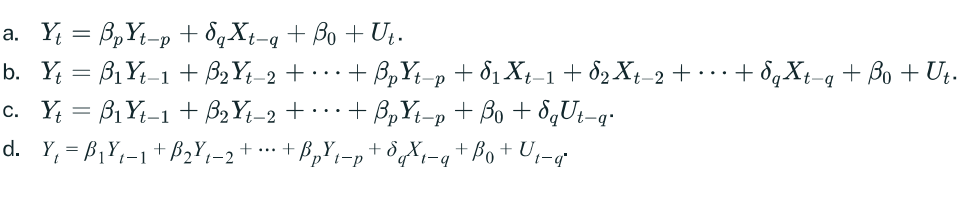
$Y_{t}=\beta_1Y_{t-1}+\beta_2Y_{t-2}+\ldots+\beta_{p}Y_{t-p}+\delta_1X_{t-1}+\delta_2X_{t-2}+\cdots$ A linear combination of lagged dependent and independent variables.

How is the root mean squared forecast error (RMSFE) defined?

$a.\sqrt{\text{E}[(Y_{T+1}-\hat{Y}_{T+1|T})^2]}$

$b.\sqrt{\text{E}[(Y_{T+1}-\hat{Y}_{T+1|T+1})^2]}$

$c.\sqrt{\text{E}[(Y_{T+1}-\hat{Y}_{T+1|T-1})^2]}$

$$\sqrt{\text{E}[(Y_{T+1}-\hat{Y}_{T+1IT})^2]}$$

Where:

$Y_{T+1}$ is the actual value at time T+1

$\hat{Y}_{T+1|T}$ is the forecast of Y_T+1​ made at time T (forecast one period ahead)

E[⋅] denotes the expected value (expectation operator)

This definition represents the theoretical or population RMSFE - it's the square root of the expected (mean) squared forecast error for one-step-ahead forecasts.

However, this differs slightly from the more common sample RMSFE I mentioned earlier, which averages over multiple actual forecast errors:

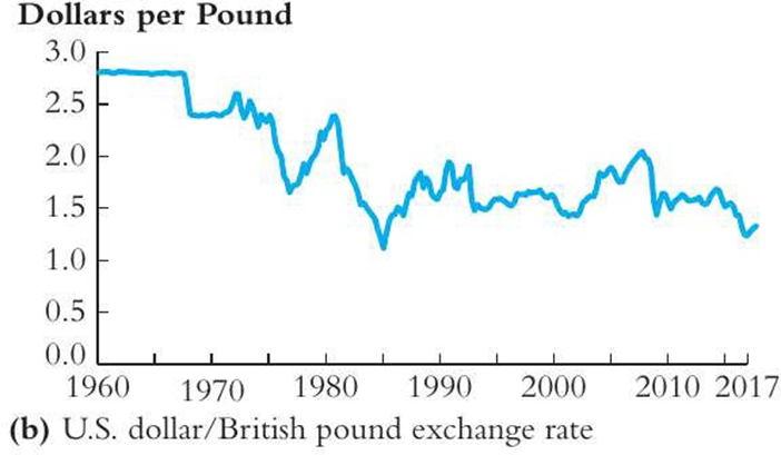
SW Figure 15.2b. Which of the following observation is true about the figure above?

a. The rate of exchange between the US dollar and the British pound experienced a structural break around 1972.

b. The rate of exchange between the US dollar and the British pound is serially uncorrelated.

c. The rate of exchange between the US dollar and the British pound exhibits strong yearly seasonal pattern.

d. There is volatility clustering in the rate of exchange between the US dollar and the British pound.

The rate of exchange between the US dollar and the British pound experienced a structural break around 1972

The 1972 exchange rate break demonstrates how structural changes invalidate econometric models. When the Bretton Woods system collapsed, the dollar-pound relationship fundamentally changed, making pre-1972 models unreliable for forecasting. This illustrates why econometricians must test for breaks using tools like the QLR statistic and verify model stability before drawing conclusions, as ignoring structural changes can lead to spurious correlations and biased predictions.

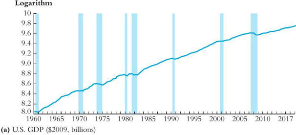
SW Figure 15.1a. Which of the following observation is true about the figure above?

a.     The log of US GDP is serially uncorrelated.

b.     The log of US GDP is increasing at a constant rate.

c.     There is an persistent upward movement in the log of US GDP.

d.     The log of US GDP has a negative autocorrelation.

 

There is an persistent upward movement in the log of US GDP.

What does the first difference of the logarithm of Yt equal?

a.     The first difference of Yt.

b.     The growth rate of Yt exactly.

c.     The difference between the lead and the lag of Yt.

d.     Approximately the growth rate of Yt when the growth rate is small.

Approximately the growth rate of Yt when the growth rate is small.

How is the Bayes-Schwarz Information Criterion (BIC) defined?

$a.BIC(p)=ln[\frac{SSR(p)}{T}]+(p+1)\cdot\frac{2}{T}$

$b.BIC(p)=ln[\frac{SSR(p)}{T}]+(p+1)\cdot\frac{\ln\left(T\right)}{T}$

$c.BIC(p)=ln[\frac{SSR(p)}{T}].(p+1)\cdot\frac{\ln\left(T\right)}{T}$

$d.BIC(p)=ln[\frac{SSR(p)}{T}]-(p+1)\cdot\frac{\ln\left(T\right)}{T}$

$$BIC(p)=ln[\frac{SSR(p)}{T}]+(p+1)\cdot\frac{\ln\left(T\right)}{T}$$

 

What is the AR(p) model?

a.     It represents Yt as a linear function of p of its lagged values.

b.     It can be written as

$Yt=\beta_1Y_{t-1}+\beta_0+U_{t-p}$

c. It is defined as

$Yt=\beta_{p}Y_{t-p}+\beta_0+U_{t}$

d.     It can be represented as:

$Y_{t}=\beta_{X}X_{t}+\beta_{p}Y_{t-p}+\beta_0+U_{t}$

 

It represents Yt as a linear function of p of its lagged values.

What characterises autoregressive distributed lag models?

a.     Current and lagged values of the error term.

b.     Lags of the dependent variable and lagged values of additional predictor variables.

c.     Lags and leads of the dependent variable.

d.     Current and lagged values of the residuals.

 

Lags of the dependent variable and lagged values of additional predictor variables.

If the AR(l) model is correct, what is a source of error in the RMSFE?

a.     Incorrectly measuring variables in logarithms.

b.     The model only looks at the previous period's value of Yt when the entire history should be taken into account.

c.     The error in estimating the coefficients \beta₁ and \beta₀.

d.     The fact that the value of the explanatory variable is not known with certainty when making a forecast.

The error in estimating the coefficients \beta₁ and \beta₀

What is a forecast?

a.     It is another word for the OLS predicted value.

b.     It is equal to the residual plus the OLS predicted value.

c.     It is close to 1.96 times the standard deviation of \(Y_t\) during the sample.

d.     It is a prediction made for some date beyond the data set used to estimate the regression.

 

It is a prediction made for some date beyond the data set used to estimate the regression.

What is the Augmented Dickey Fuller (ADF) t-statistic?

a.     It has the identical distribution whether or not a trend is included or not.

b.     It has a normal distribution in large samples.

c.     It is an extension of the Dickey-Fuller test when the underlying model is AR(p) rather than AR(l).

d.     It is a two-sided test.

It is an extension of the Dickey-Fuller test when the underlying model is AR(p) rather than AR(l).

What is a reason for computing the logarithms, or changes in logarithms, of economic time series?

a.     Natural logarithms are easier to work with than base 10 logarithms.

b.     Numbers often get very large.

c.     They often exhibit growth that is approximately exponential.

d.     Economic variables are hardly ever negative.

They often exhibit growth that is approximately exponential.

What happens if a "break" occurs in the population regression function?

a.     This suggests the presence of a deterministic trend in addition to a stochastic trend.

b.     An Augmented Dickey Fuller test, rather than the Dickey Fuller test, should be used to test for stationarity.

c.     Forecasting, but not inference, is unaffected, if the break occurs during the first half of the sample period.

d.     Then inference and forecasting are compromised when neglecting it.

Then inference and forecasting are compromised when neglecting it.

What does negative autocorrelation in the change of a variable imply?

a.     The series is not stable over time.

b.     An increase in the variable in one period is, on average, associated with a decrease in the next.

c.     The data is negatively trended.

d.     The variable contains only negative values.

An increase in the variable in one period is, on average, associated with a decrease in the next.

How can we characterise the linear probability model?

a. It is the application of the linear multiple regression model to a binary dependent variable.

b. It is an example of probit estimation.

c. It is another word for logit estimation.

d. It is the application of the multiple regression model with a continuous left-hand side variable and a binary variable as at least one of the regressors.

It is the application of the linear multiple regression model to a binary dependent variable.

What is a property of the probit model?

a. It is the same as the logit model.

b. It always gives the same fit for the predicted values as the linear probability model for values between 0.1 and 0.9.

c. It forces the predicted values to lie between 0 and 1.

It forces the predicted values to lie between 0 and 1.

What is true of nonlinear least squares estimation?

a.     Is another name for sophisticated least squares.

b.     Solves the minimisation of the sum of squared predictive mistakes.

c.     Should always be used when you have nonlinear equations.

d. Gives you the same results as maximum likelihood estimation.

Solves the minimisation of the sum of squared predictive mistakes.

In the linear probability model, what is the interpretation of the linear slope coefficient?

a.     The change in probability that Y = 1 associated with a unit change in X, holding others regressors constant.

b.     Not all that meaningful since the dependent variable is either 0 or 1.

c.     The change in odds associated with a unit change in X, holding other regressors constant.

d. The response in the dependent variable to a percentage change in the regressor.

The change in probability that Y = 1 associated with a unit change in X, holding others regressors constant.

Which one of the following cannot be analysed using probit and logit estimation?

a. Whether a college student decides to study abroad for one semester.

b. Whether applicants will default on a loan.

c. Whether being a female has an effect on earnings.

d. Whether a college student will attend a certain college after being accepted.

Whether being a female has an effect on earnings.

In the expression $P(Y=1|X)=\Phi(\beta1X+\beta0)$ , which of the following fact about $β_1X+β_0$ is true?

a. $\beta_1 X + \beta_0$ plays the role of z in the cumulative standard normal distribution function.

b. $\beta_0$ cannot be negative since probabilities have to lie between 0 and 1.

c. $\beta_1$ cannot be negative since probabilities have to lie between 0 and 1.

d. $\beta_1 X + \beta_0 > 0$ since probabilities have to lie between 0 and 1.

$\beta_1 X + \beta_0$ plays the role of z in the cumulative standard normal distribution function.

What is a property of coefficients estimated by the maximum likelihood method?

a. They are typically larger than those from OLS estimation.

b. They come from a probability distribution and hence have to be positive.

c. They minimise the sum of squared prediction errors.

d. They maximise the likelihood function.

They maximise the likelihood function.

What does the coefficient β on X indicate in a probit regression?

The change in the probability of Y=1 given a unit change in X.

The change in the z-value associated with a unit change in X.

The change in the probability of Y=1 given a percent change in X.

SW equation 11.8. Using the estimated probit model above, answer the following question: Suppose a black mortgage applicant reduced her P/I ratio from 0.42 to 0.34. What effect would this have on her probability of being denied a mortgage?

Her probability of being denied a mortgage increases by 7.67 percentage points.

Her probability of being denied a mortgage decreases by 5.14 percentage points.

Her probability of being denied a mortgage decreases by 7.67 percentage points.

Not enough information to determine the effect.

Her probability of being denied a mortgage decreases by 7.67 percentage points.

SW equation 11.8. Using the estimated probit model above, answer the following question: Suppose a white mortgage applicant has a P/IP/I ratioratio of 0.38. What is the estimated probability that her applicant will be denied?

22.81 percentage points.

11.15 percentage points.

48 percentage points.

27.4 percentage points.

11.15 percentage points.

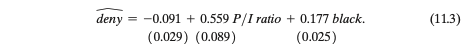
SW equation 11.3. Which of the following is a correct interpretation of the estimated coefficient on P/IP/I ratioratio?

An increase in P/IP/I ratioratio by 0.03 is associated with an increase in the probability of mortgage denial by 1.877 percentage points, holding race constant.

A decrease in P/IP/I ratioratio by 0.01 is associated with an increase in the probability of mortgage denial by 0.559 percentage points, holding race constant.

An increase in P/IP/I ratioratio by 0.01 is associated with a decrease in the probability of mortgage denial by 0.559 percentage points, holding race constant.

An increase in P/IP/I ratioratio by 0.02 is associated with an increase in the probability of mortgage denial by 1.118 percentage points, holding race constant.

An increase in P/I ratio by 0.02 is associated with an increase in the probability of mortgage denial by 1.118 percentage points

• Change = 0.559 × 0.02 = 0.01118 = 1.118 percentage points

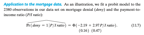
SW equation 11.7. Which of the following is a correct interpretation of the estimated coefficient on P/IP/I ratioratio?

An increase in P/IP/I ratioratio by 0.01 is associated with a decrease in the probability of mortgage denial by 2.97 percentage points.

The probability of mortgage denial given P/IP/I ratioratio = 1 is 29.7 percentage points.

P/IP/I ratioratio is positively related to the probability of mortgage denial.

An increase in P/IP/I ratioratio by 0.01 is associated with an increase in the probability of mortgage denial by 2.97 percentage points.

In a probit model, the coefficients don't directly represent marginal effects on probabilities. Instead, they represent the effect on the z-value (the argument inside the cumulative normal distribution function Φ).

"P/I ratio is positively related to the probability of mortgage denial."

• This is correct. The coefficient 2.97 is positive, meaning that as P/I ratio increases, the z-value increases, which increases Φ(z-value), thus increasing the probability of denial.

In the binary dependent variable model, what does a predicted value of 0.6 mean?

a. Given the values for the explanatory variables, there is a 40 percent probability that the dependent variable will equal one.

b. The most likely value the dependent variable will take on is 60 percent.

c. The model makes little sense, since the dependent variable can only be 0 or 1.

d. Given the values for the explanatory variables, there is a 60 percent probability that the dependent variable will equal one.

Given the values for the explanatory variables, there is a 60 percent probability that the dependent variable will equal one.

What does the logit model derive its name from?

a.

The logistic function.

b.

The logarithmic function.

c.

The log-linear relationship.

The logistic function.

Consider the expression

$$P(deny=1|pi_{ratio,black})=\Phi(–2.26+2.74pi_{ratio}+0.71black)$$

What is the effect of increasing the P/I ratio from 0.3 to 0.4 for a white person?

a.

It is 4.7 percentage points.

b.

It is 0.274 percentage points.

c.

It is 6.1 percentage points.

d.

It is 2.74 percentage points.

It is 4.7 percentage points.

What does the expression $E(Y|X1,…,Xk)=P(Y=1|X1,…,Xk)$ mean?

You are pretty certain that Y takes on a value of 1 given the Xs.

For a binary variable model, the predicted value from the population regression is the probability that Y=1given X.

Dividing YY by the XXs is the same as the probability of YY being the inverse of the sum of the XX's.

The exponential of YY is the same as the probability of YY happening.

For a binary variable model, the predicted value from the population regression is the probability that Y=1given X.

What can be considered a flaw of the linear probability model?

a.

The predicted values can lie above 1 and below 0.

b.

The regression R2R2 cannot be used as a measure of fit.

c.

The observed values can only be 0 and 1, but the predicted are almost always different from that.

The predicted values can lie above 1 and below 0.

How are probit coefficients typically estimated?

a.

By transforming the estimates from the linear probability model.

b.

Using the method of maximum likelihood.

c.

Using non-linear least squares.

d.

By the ordinary least squares method.

Using the method of maximum likelihood.

In the probit model $P(Y=1|X)=Φ(β1X+β0)$ , what is Φ?

a.

It is the standard normal cumulative distribution function.

b.

It is set to 1.96.

c.

It is not defined for Φ(0)Φ(0).

d.

It can be computed from the standard normal density function.

It is the standard normal cumulative distribution function.

What is true about the probit model

$P(Y=1|X1,X2,…,Xk)=Φ(β1X1+β2X2+⋯+βkXk)$ ?

a.β₀ is the probability of observing YY when all XXs are 0.

b.β₀ cannot be negative since probabilities have to lie between 0 and 1.

c. The βs do not have a simple interpretation.

d. The slopes tell you the effect of a unit increase in X on the probability of Y.

The βs do not have a simple interpretation.

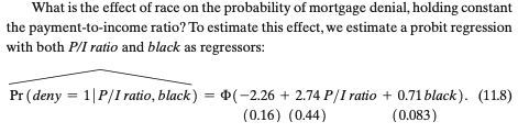
SW equation 11.8. Using the estimated probit model above, answer the following question: Suppose a white mortgage applicant increased her P/IP/I ratioratio from 0.26 to 0.34. What effect would this have on her probability of being denied a mortgage?

a. Her probability of being denied a mortgage increases by 3.4 percentage points.

b. Her probability of being denied a mortgage decreases by 3.12 percentage points.

c. Not enough information to determine the effect.

d. Her probability of being denied a mortgage increases by 3.12 percentage points.

At P/I ratio = 0.26: z-value = -2.26 + 2.74(0.26) = -2.26 + 0.7124 = -1.5476 Pr(deny = 1) = Φ(-1.5476) ≈ 0.061 = 6.1%

At P/I ratio = 0.34: z-value = -2.26 + 2.74(0.34) = -2.26 + 0.9316 = -1.3284 Pr(deny = 1) = Φ(-1.3284) ≈ 0.092 = 9.2%
Her probability of being denied a mortgage increases by 3.12 percentage points.

SW equation 11.10. Which of the following is a correct interpretation of the estimated coefficient on black?

a. The probability of mortgage denial for an African American applicant is 1.27 percentage points higher than the probability of mortgage denial for a white applicant, holding P/I ratio constant.

b. An African American applicant has a higher probability of mortgage denial than a white applicant, holding P/I ratio constant.

c. The probability of mortgage denial for an African American applicant is 0.781 percentage points higher than the probability of mortgage denial for a white applicant, holding P/I ratio constant.

d. An African American applicant has a lower probability of mortgage denial than a white applicant, holding P/I ratio constant.

"An African American applicant has a higher probability of mortgage denial than a white applicant, holding P/I ratio constant."

• This is correct. The coefficient on black is positive (1.27), which means that being African American increases the argument of the logistic function, thereby increasing the probability of denial.

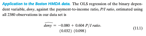
SW equation 11.1. Which of the following is a correct interpretation of the estimated coefficient on P/IP/I ratioratio?

a. An increase in P/IP/I ratioratio by 0.01 is associated with a decrease in the probability of mortgage denial by 0.604 percentage points.

b. A decrease in P/IP/I ratioratio by 0.01 is associated with an increase in the probability of mortgage denial by 0.604 percentage points.

c. The probability of mortgage denial given P/IP/I ratioratio = 1 is 60.4 percentage points.

d. An increase in P/IP/I ratioratio by 0.03 is associated with an increase in the probability of mortgage denial by 1.812 percentage points.

An increase in P/I ratio by 0.03 is associated with an increase in the probability of mortgage denial by 1.812 percentage points.

• Change = 0.604 × 0.03 = 0.01812 = 1.812 percentage points

SW equation 11.8. Using the estimated probit model above, answer the following question: Suppose a black mortgage applicant has a P/IP/I ratioratio of 0.38. What is the estimated probability that her applicant will be denied?

a. 11.9 percentage points.

b. 27.4 percentage points.

c. 37.55 percentage points.

d. 30.54 percentage points.

What is the formula for the first stage in AP's charter schools IV example?

Question 1Answer

a. Effect of offers on attendance=Effect of offers on scores / Effect of attendance on scores

b. Effect of offers on attendance=Effect of attendance on scores / Effect of offers on scores

c. Effect of offers on attendance=Effect of offers on scores × Effect of attendance on scores

Effect of offers on attendance=Effect of offers on scores / Effect of attendance on scores

Assuming monotonicity, who is the average treatment effect (ATE) for?

a. Compliers.

b. Never-takers.

c. Always-takers.

d. Defiers.

Compliers

Which of the following would violate the independence assumption in AP's charter schools IV example?

a. Some lottery losers attend the charter school.

b. Offers are given based on family income instead of lottery.

c. Offers are randomly assigned.

d. Not all lottery winners attend the charter school.

Offers are given based on family income instead of lottery.

What is the formula for the reduced form in AP's charter schools IV example?

a. Effect of offers on scores=Effect of attendance on scores / Effect of offers on attendance

b. Effect of offers on scores=Effect of offers on attendance × Effect of attendance on scores

c. Effect of offers on scores=Effect of offers on attendance / Effect of attendance on scores

Effect of offers on scores=Effect of offers on attendance×Effect of attendance on scores

In AP's charter schools IV example, what gives us the independence assumption?

a. Charter schools are free to structure their curricula and school environments.

b. Lottery winners are not related to the teachers in the charter school.

c. Lottery outcomes are randomly assigned.

d. Lottery losers are prohibited from attending the charter school.

Lottery outcomes are randomly assigned.

In AP's charter schools IV example, what effect is being investigated?

a. The effect of charter school offers on school achievement.

b. The effect of charter school attendance on school achievement.

c. The effect of charter school attendance on school achievement differences across race.

d. The effect of charter school offers on charter school attendance.

The effect of charter school attendance on school achievement.

What method is used to establish identification of the causal parameter in IV models?

a. Methods of least squares.

b. Methods of maximin.

c. Method of minimax.

d. Method of moments.

Method of moments.

As in the lecture notes, let $Y_i,D_i,O_i,Z_i$ be random variables representing an outcome, a treatment, control variables, and instruments. Suppose

$Yi=γ1Di+γ′2Oi+γ0+Vi$ and$Di=π′1Zi+π′2Oi+π0+Wi$
What is a condition for Z_i being a valid instrument?

a. $\gamma_1\ne0$

b. $\gamma_0\ne0$

c. $\pi_1\ne0$

d. $\pi_0\ne0$

$$\pi_0\ne0$$

How can we check the instrument relevance assumption?

a. It is not possible to verify the relevance assumption statistically.

b. We can check that the F statistic for the coefficient on the instrument in first stage is larger than 10.

c. We can check that the coefficient on the instrument in the first stage is significant.

d. We can check that the coefficient on the treatment variable in the second stage is significant.

We can check that the F statistic for the coefficient on the instrument in first stage is larger than 10.

What does selection on unobservables mean?

a. There is an unobserved component to potential outcomes.

b. The treatment variable is partly unobserved.

c. Conditioning on unobservables cannot make potential outcomes and assignment to treatment independent.

d. Conditioning on observables cannot make potential outcomes and assignment to treatment independent.

Conditioning on observables cannot make potential outcomes and assignment to treatment independent.

What is the problem of doing two-stage estimation in two stages?

a. The estimation error in the second stage affects the first stage.

b. The standard errors in the second stage are wrong.

c. The estimator of the causal parameter is inconsistent.

d. The selection bias is not eliminated.

The standard errors in the second stage are wrong.

As in the lecture notes, let Y_i,D_i,O_i,Z_i be random variables representing an outcome, a treatment, control variables, and instruments. Also let V_i be the error term in the structural equation and let W_i be the error term in the first stage equation. What is a condition for Z_i being a valid instrument?

$E(Vi$E(Wi|Zi,Oi)=0$$E(Vi|Zi,Oi)=0$$E(Wi|Di,Oi)=0$$

$$E(Vi|Zi,Oi)=0$$

What is the instrumental variable used in AP's charter schools IV example?

a. A dummy variable indicating lottery winners who attend the charter school.

b. Student math and verbal scores.

c. A dummy variable indicating KIPP applicants who won the lottery.

d. A dummy variable indicating KIPP applicants who are eligible for the federal government's subsidised lunch program.

A dummy variable indicating KIPP applicants who won the lottery.

What is the instrument relevance assumption in AP's charter schools IV example?

Question 2Answer

a. Lottery outcome must have an effect on student achievement.

b. Lottery outcome must not have an effect on student achievement.

c. Lottery outcome must have an effect on charter school attendance.

d. Lottery outcomes are randomly assigned.

Lottery outcome must have an effect on charter school attendance.

Following the notation in Chapter 3.1 of AP, which of the following represents the LATE?

$$(E[Yi|Zi=1]−E[Yi|Zi=0])×(E[Di|Zi=1]−E[Di|Zi=0])$$

$$\frac{(E[Di|Zi=1]-E[Di|Zi=0])}{(E[Yi|Zi=1]-E[Yi|Zi=0])}$$

$$\frac{(E[Yi|Zi=1]-E[Yi|Zi=0])}{(E[Di|Zi=1]-E[Di|Zi=0])}$$

$$\frac{(E[Yi|Zi=1]-E[Yi|Zi=0])}{(E[Di|Zi=1]-E[Di|Zi=0])}$$

What is the exclusion restriction assumption in AP's charter schools IV example?

a. Lottery outcomes are randomly assigned.

b. Lottery outcome must have an effect on charter school attendance.

c. Lottery outcome must not have an effect on student achievement.

d. Lottery losers must not attend the charter school.

Lottery outcome must not have an effect on student achievement.

Following the notation in Chapter 3.1 of AP, which of the following represents the first stage?

$$E[Z_i|D_i=1]-E[Z_i|D_i=0]$$

$$E[Y_i|D_i=1]-E[Y_i|D_i=0]$$

$$E[D_i|Z_i=1]-E[D_i|Z_i=0]$$

$$E[Y_i|Z_i=1]- E[Y_i|Z_i=0]$$

$$E[D_i|Z_i=1]-E[D_i|Z_i=0]$$

Who are the compliers in AP's charter schools IV example?

a. Students who attend the charter school regardless of being offered or not.

b. Students who attend the charter school when offered but do not attend when not offered.

c. Students who do not attend the charter school when offered but attend the charter school when not offered.

d. Students who do not attend the charter school regardless of being offered or not.

Students who attend the charter school when offered but do not attend when not offered.

As in the lecture notes, let Yi,Di,Oi,ZiYi,Di,Oi,Zi be random variables representing an outcome, a treatment, control variables, and instruments. Suppose all conditional mean functions are linear. What is the structural equation?

$$Y_i=δ^′_1Z_i+δ^′_2O_i+δ_0+Ui$$

$$Y_i=γ_1D_i+γ^′_2O_i+γ_0+V_i$$

$$Di=π′1Zi+π′2Oi+π0+Wi$$

$$Y_i=\beta^′_1D_i+\beta^′_2O_i+\beta^′_3Z_i+\beta_0+U_i$$

$$Y_i=γ_1D_i+γ^′_2O_i+γ_0+V_i$$

What happens if the coefficient on the instrument in the first stage is 0?

a. Identification of the causal parameter fails.

b. The standard errors of the estimated causal parameter become very small.

c. The selection bias is eliminated.

d. The reduced form parameter and the causal parameter are the same.

Identification of the causal parameter fails.

What is an endogenous variable?

a. A variable that is uncorrelated with the error term in the first stage.

b. A variable that appears in the first stage equation.

c. A variable that is correlated with the error term in the structural equation of interest.

d. A variable that is determined outside the model.

A variable that is correlated with the error term in the structural equation of interest.

As in the lecture notes, let Yi,Di,Oi,ZiYi,Di,Oi,Zi be random variables representing an outcome, a treatment, control variables, and instruments. Suppose all conditional mean functions are linear. What is the first stage equation?

a.$Y_i=δ^′_1Z_i+δ^′_2O_i+δ_0+U_i$

b.$Y_i=β_1D_i+β^′_2O_i+β^′_3Z_i+β_0+U_i$

c. $Y_i=γ_1D_i+γ^′_2O_i+γ_0+V_i$

d. $D_i=π^′_1Z_i+π^′_2O_i+π_0+W_i$

$$D_i=π^′_1Z_i+π^′_2O_i+π_0+W_i$$

What does selection on observables mean?

a. Conditioning on observables makes potential outcomes and assignment to treatment independent.

b. The instrumental variable is observed without measurement error.

c. Assignment to treatment is based on observed variables, as opposed to randomisation.

d. Potential outcomes are fully determined by observed variables.

What is a reason we might need to include control variables when we use IV estimation?

a. We like to include regressors in order to improve the fit of the model.

b. We want to include regressors in order reduce the standard error of the causal parameter.

c. We need to capture that treatment is assigned with different probabilities for different values of control variables.

d. Including control variables makes the first stage stronger.

We need to capture that treatment is assigned with different probabilities for different values of control variables.

In the DD analysis of bank run in Mississippi, what is the dilemma?

a. Whether to merge troubled banks.

b. Whether to renew licenses of troubled banks.

c. Whether to bail out troubled banks.

d. Whether to increase the interest rate.

Whether to bail out troubled banks.

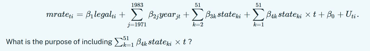
Consider the model

Record

a. To reduce the risk of omitted variable bias.

b. To allow for non-parallel trends across states.

c. To improve the precision the causal effect of a reduction the minimum legal drinking age on mortality rate.

d. To account for potential fixed differences in mortality rate across states.

To allow for non-parallel trends across states.

In the DD analysis of the minimum legal drinking age in the U.S., why do we include dummy variables for years?

a. To reduce the risk of omitted variable bias.

b. There may be changes in mortality rate over time that occur in all states.

c. To adjust for correlation in the standard errors.

d. To determine the time-specific causal effect of a reduction in the minimum legal drinking age.

There may be changes in mortality rate over time that occur in all states.

Which of the following is a key assumption in DD analysis?

a. The level of the dependent variable for the treatment and control groups are the same prior to the treatment.

b. The trends are smooth.

c. During non-treatment periods, the trend of the treatment and control groups are not the same.

d. Other than the treatment, nothing else affected the treatment and control groups differently.

Other than the treatment, nothing else affected the treatment and control groups differently.

Following the notation in AP 5.1, what is the equation for the DD estimate δ_DD of the effect of increased lending?

a.

$$\delta_{DD}=(Y_{6,1931}+Y_{6,1930})-(Y_{8,1931}+Y_{6,1931})$$

$$\delta_{DD}=(Y_{8,1931}-Y_{8,1930})$$

$$\delta_{DD}=(Y_{6,1931}-Y_{6,1930})$$

$$\delta_{DD}=(Y_{8,1930}-Y_{6,1930})-(Y_{8,1931}-Y_{6,1931})$$

$$\delta_{DD}=(Y_{8,1930}-Y_{6,1930})-(Y_{8,1931}-Y_{6,1931})$$

Define four categorical variables$Cgp_i=1(G_i=g,P_i=p)$ where 1(⋅) denotes the indicator function and G_i and P_i are dummy variables. Suppose

$E(Y_i|G_i,P_i)=\beta1C01_i+\beta2C10_i+\beta3C11_i+\beta_0$
What is the interpretation of β₀?

a. The difference in the average of Y_i between observations with G_i=0,P_i=0 and observations with G_i=1,P_i=0.

b. The average of Y_i for observations with G_i=1,P_i=1.

c. The difference in the average of Y_i between observations with G_i=0,P_i=0 and observations with G_i=1, P_i=1.

d. The average of Y_i for observations with G_i=0,P_i=0.

The average of Y_i for observations with G_i=0, P_i=0.

In DD analysis, why do we compare changes instead of levels?

a. Because changes are more interesting to look at.

b. Because levels have omitted variable bias.

c. To account for the fact that the treatment and control groups may have different values to begin with.

d. To allow for differences in the treatment effect.

To account for the fact that the treatment and control groups may have different values to begin with.

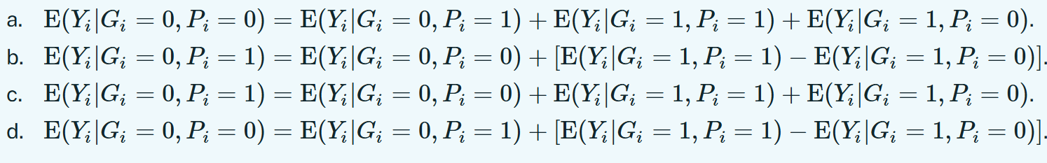
Suppose Y_i is a random outcome variable and G_i and P_i are dummy variables. Which of the following equations reflects the common trends assumption?

b

Define four categorical variables$Cgp_i=1(G_i=g,P_i=p)$ where 1(⋅) denotes the indicator function and G_i and P_i are dummy variables. Suppose

$E(Y_i|G_i,P_i)=\beta_1C01_i+\beta_2C10_i+\beta_3C11_i+\beta_0$
What is the interpretation of β₁?

a. The difference in the average of Y_i between observations with G_i=0, P_i=1 and observations with G_i=1,P_i=1.

b. The average of Y_i for observations with G_i=0,P_i=1.

c. The difference in the average of Y_i between observations with G_i=0,P_i=1 and observations with G_i=1, P_i=0.

d. The difference in the average of Y_i between observations with G_i=0,P_i=1 and observations with G_i=0, P_i=0.

The difference in the average of Y_i between observations with G_i=0,P_i=1 and observations with G_i=0, P_i=0.

What does the dashed line in Figure 5.1 of AP 5.1 represent?

a. The outcome that would have happened if the 6th district did not experience increased lending.

b. The expected causal effect of increased lending in the 6th district.

c. The outcome that would have happened if the 6th district did not experience the same number of bank failures as in the 8th district.

d. The outcome that would have happened if the 8th district experienced increased lending.

The outcome that would have happened if the 6th district did not experience increased lending.

In the DD analysis of the minimum legal drinking age in the U.S., why do we include dummy variables for states?

a. To determine the state-specific causal effect of a reduction in the minimum legal drinking age.

b. To ensure that the state-specific time trends are parallel.

c. To account for potential fixed differences in mortality rate across states due to systematic differences (cultural, geographical, etc.).

d. To reduce the risk of omitted variable bias.

To account for potential fixed differences in mortality rate across states due to systematic differences (cultural, geographical, etc.).

Suppose that there are four sub-populations (group 0 in period 0, group 0 in period 1, group 1 in period 0, group 1 in period 1), where neither group is treated in period 0 and Group 1 is treated in period 1. Let YiYi be the dependent variable, GiGi be the group variable that takes values 0 or 1, and PiPi be the period variable that also takes values 0 or 1. The linear regression model for the DD research design is

$$E(Yi|Gi,Pi)=αGi+βPi+δGi⋅Pi+κ .$$

What is the DD causal effect of treatment?

a. δ+κ

b. δ

c. δ−β

d. δ−α

δ

How can the plausibility of the common trends assumption be tested?

a. Compare the level of the dependent variable for the treatment and control groups prior to the treatment.

b. Compare the characteristics of the treatment and control groups prior to the treatment.

c. Compare the trend for the treatment group before and after the treatment.

d. Compare the trend for the treatment and control groups during periods where both are untreated.

Compare the trend for the treatment and control groups during periods where both are untreated.

Which of the following is a key assumption in DD analysis?

a. The treatment and control groups have similar characteristics prior to the treatment.

b. The evolution of the dependent variable would be the same for both the treatment and control groups in the absence of treatment.

c. The level of the dependent variable for the treatment group is different from that of the control group after the treatment.

d. The treatment and control groups are selected randomly.

The evolution of the dependent variable would be the same for both the treatment and control groups in the absence of treatment.

Suppose YiYi is a random outcome variable and GiGi and PiPi are dummy variables. Which of the following equations reflects the common trends assumption?

$$ATT=[E(Yi|Gi=1,Pi=1)−E(Yi|Gi=0,Pi=1)]−[E(Yi|Gi=1,Pi=0)−E(Yi|Gi=0,Pi=0)]$$

$$ATT=[E(Yi|Gi=1,Pi=1)+E(Yi|Gi=0,Pi=1)]−[E(Yi|Gi=1,Pi=0)+E(Yi|Gi=0,Pi=0)]$$

$$ATT=[E(Yi|Gi=0,Pi=1)−E(Yi|Gi=1,Pi=0)]−[E(Yi|Gi=0,Pi=0)−E(Yi|Gi=1,Pi=1)]$$

$ATT=[E(Yi|Gi=1,Pi=1)−E(Yi|Gi=0,Pi=1)]$ $−[E(Yi|Gi=1,Pi=0)−E(Yi|Gi=0,Pi=0)]$

In the DD analysis of bank run in Mississippi if in addition to the treatment, the 6th district also discovered new raw materials (oil reserves) during treatment periods, why would that affect the validity of interpreting the DD estimate as the causal effect of increased lending?

a. We wouldn't be able to tell if the DD estimate is the effect of the increased lending or the discovery of new raw materials (or both).

b. There could be omitted variable bias due to the discovery of new raw materials.

c. The trends are not parallel.

d. The causal effect of the discovery of new raw materials may outweigh the causal effect of increased lending.

We wouldn't be able to tell if the DD estimate is the effect of the increased lending or the discovery of new raw materials (or both).

Table 5.1 of AP 5.1, suppose that the common trends assumption hold for the number of wholesale firms, what is the DD estimate of the causal effect of increased lending on the number of wholesale firms?

a. -323.

b. 181.

c. 34.

d. -147.

e. -142.

181

Table 5.1 of AP 5.1, suppose that the common trends assumption hold for the net wholesale sales ($ million), what is the DD estimate of the causal effect of increased lending on the net wholesale sales ($ million)?

a. -104.

b. -81.

c. -162.

d. 81.

e. -23.

81

In the DD analysis of bank run in Mississippi, what is the treatment being examined?

a. Increased lending to troubled banks.

b. Increased number of banks.

c. Increased interest rate.

d. Decreased lending to troubled banks.

Increased lending to troubled banks.

Practically, how is DD implemented?

a. Using instrumental variables.

b. Through regression analysis.

c. By including control variables that explain the regressand and may be correlated with the regressors.

d. Through randomised control trials.

Through regression analysis.

In the DD analysis of bank run in Mississippi, if the treatment is effective, what outcome would we expect to observe?

a. Decrease in bank failures.

b. Increase in bank failures.

c. No bank failures.

d. Bank failures remain constant.

Decrease in bank failures.

In the DD analysis of bank run in Mississippi, what is the dilemma?

a. Whether to increase the interest rate.

b. Whether to merge troubled banks.

c. Whether to renew licenses of troubled banks.

d. Whether to bail out troubled banks.

Whether to bail out troubled banks.

Which of the following is a key assumption in DD analysis?

a. Other than the treatment, nothing else affected the treatment and control groups differently.

b. The level of the dependent variable for the treatment and control groups are the same prior to the treatment.

c. During non-treatment periods, the trend of the treatment and control groups are not the same.

d. The trends are smooth.

Other than the treatment, nothing else affected the treatment and control groups differently.

In DD analysis, why do we compare changes instead of levels?

a. To allow for differences in the treatment effect.

b. To account for the fact that the treatment and control groups may have different values to begin with.

c. Because levels have omitted variable bias.

d. Because changes are more interesting to look at.

To account for the fact that the treatment and control groups may have different values to begin with.

What is the purpose of the peer group model?

a. To study whether the average SAT scores of the peer group matters for future earnings.

b. To see if the SAT scores tend to be higher at private universities.

c. To disentangle the influence of peer groups from the influence of attending a private university on future earnings.

d. To investigate if students prefer universities where the other students have similar SAT scores.

To study whether the average SAT scores of the peer group matters for future earnings. (probably)

Suppose we group students by the set of universities they applied to and were admitted to. Looking across groups, what is the main reason for the differences in average earnings?

a. Differences in the proportion who attended a private university.

b. Differences in the students' average ambition and ability.

c. The causal effect of applying and being admitted to particular universities.

Differences in the students' average ambition and ability.

How do the estimates from the self-revelation model compare with those using Barron matches?

a. The estimates are much more sensitive to the inclusion of other control variables in the self-revelation model.

b. The estimated gap between studying at a private and a public university are lower in the self-revelation model.

c. Both suggests that studying at a private university has little effect on future earnings.

d. The precision of the estimates is much higher in the self-revelation model.

Both suggests that studying at a private university has little effect on future earnings.

Suppose $E(Y|T,A)=\beta_1T+\beta_2A+\beta_0$ where Y is earnings, A is a group indicator (0 or 1), and T is a treatment indicator (0 or 1). If $β_2=60,000$, what is the implication?

a. People in group 1 earn 60,000 dollars more than those in group 0, holding A constant.

b. People in group 1 earn 60,000 dollars more than those in group 0, holding T constant.

c. Treated people earn 60,000 dollars more than untreated people, holding T constant.

d. Treated people earn 60,000 dollars more than untreated people, holding A constant.

People in group 1 earn 60,000 dollars more than those in group 0, holding T constant.