BIN300 - W8 Non-linear models for genomic selection and QTL mapping

assumption in GBLUP/SNP-BLUP mode

SNPs have normal distribution with equal simga²

not realistic, because some SNPs probably have very big effect, many SNPs have little or no effect, kurtosis > 0 (normal distribtuion kurtosis = 0)

use non-normal prior distribution (t,exponential, etc)

• SNP effects depend on whether they are close to a gene or not

•

• Gene effects often are believed to be exponential or gamma distributed in the evolutionary literature.

kurtosis, normal distribution

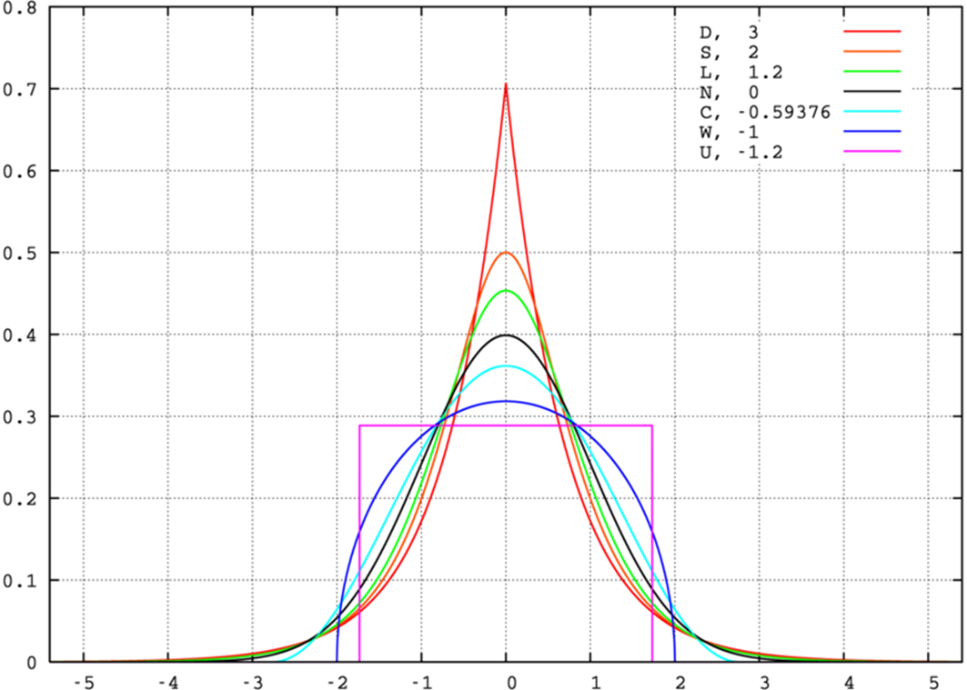
• distributions with high kurtosis (red) are more peaked in the centre and have a higher probability at the tails, i.e. there are many more genes with little effect but also some more with very big effects (eg 4-5 standard deviations).

•

• Red curve is for the Double-Exponential distribution (see next slide)

Non-linear GS methods

BayesA,B,C, Bayesian lasso, lasso

A: t-distribution

B: with probability pie: t distribution, with probablity (1-pie): 0

C: with pobability pie: normal distribution, with porb (1-pie): 0

bayesian lasso: double-exponential DE Distr.

lasso: DE prior, uses mode instead of mean

•for comparison: GBLUP uses the Normal distribution as prior for the SNP effects

•

•For t-distribution often 4.1 degrees of freedom are used (as was derived in the original paper by Meuwissen et al. 2001; Genetics 157). Note: degrees_of_freedom=4 gives a t-distribution with infinite kurtosis. Df=4.1 gives a kurtosis of 60.

•

•BayesB and BayesC assume that many SNPs are not close to a QTL, and thus that many QTL effects are truly 0.

•

• the ’mode’ is the top of the distribution, ie. the most probable value, instead of the mean which is the average value. For non-linear skewed distributions, the mode differs from the mean. Due to the use of the mode, the (normal) Lasso results in many SNP effects being set to 0, which may be an advantage since they then do not need to be genotyped in the animals whose breeding values are evaluated.  

•

differneces between GBLUP, Bayes A,B,C, Bayesion lasso

Two groups of methods: GBLUP, Bayes A, Bayesian Lasso

• different prios, but all SNPs have effects

Bayes B,C,

• Many SNP effects are assumed to be 0

in sumulations: Bayes B/Bayes C perform better

in real data: basyesB/C marginally better, often not much difference

• It is often thought that the real data contain more QTL than the simulated data such that the assumption of all SNPs having an effect becomes true.

•

•Also the use of (too) low marker density in practice can result in that the QTL effects are distributed over many SNPs that are in partial LD with the QTL. Thus, many SNPs need to be fitted to explain the QTL and the prior assumption that all SNPs need to be fitted is pretty good.

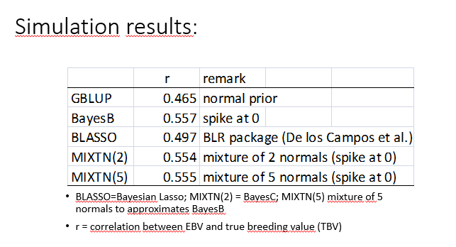
simulation results

• Simulation: 1 chromosome (100 cM); 30 QTL; 1000 SNPs, 200 phenotyped and genotyped animals to estimate SNP effects (training animals). Predicted are animals that are outside these 200 animals and are only genotyped.

•

•R=

•

• Assuming that many SNP effects are 0, implies that there is a spike at 0 when one plots the prior distribution.

•

•Methods without spike at 0 have accuracy 0.46-0.50 (here)

•

•Methods with spike at 0 have accuracy around 0.55 (here)

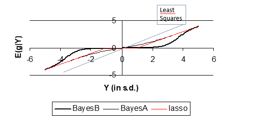
non-linear regression

• graph plots ’signal for a SNP effect’ (which is the least-square mean of the SNP effect) against the estimated effect. Thus, least-squares regression would result in a straight line with a slope of 1. GBLUP results in a straight line with a slope less than 1 (BLUP regresses the estimates back to 0).

•

•BayesA yields a non-linear curve, but it is close to linear.

•

•The Lasso results in a ’broken stick’ curve: close to Y=0 all estimates are set to zero (the Lasso believes that small Y values are due to random noise and sets the estimate to 0). But if the signal exceeds a threshold (Y≈1) here, the Lasso starts to believe that the SNP effect is real and yields an estimate >0.

•

•BayesB does this same as the Lasso, but in a more extreme way and without the fixed thresholds, ie. the curve changes gradually (no broken curve).

•

•BayesA does the same as the Lasso, but in a less extreme way and again the curve makes only gradual changes.       

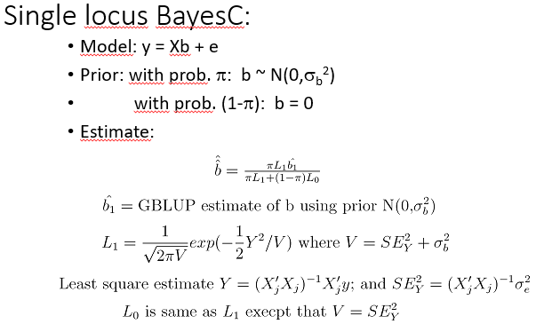
SIgnle locus Bayes C

• BayesC is worked out here since it is perhaps the easiest of the ’spike at 0’ methods and is usually as good as BayesB, which is more complicated.

•

•BayesC may be seen as a mixture of normal distributions, where one of the normal distribution has variance 0.

•

• BayesC estimate is thus a further regressed back GBLUP estimate, where the regression coefficient depends on the posterior probability (= prior probability * likelihood) of the SNP having a real effect.

•

•The likelihood is calculated here using the least square estimate of the SNP effect (Y). It could also have been calculated using the multivariate normal distribution which is proportional to |V|^-0.5exp(-0.5y’V^-1y), where y= vector of records; V=variance covariance matrix of records; V=X_jX_j’*σ_b²+I*σ_e².

M

Many-loci BayesC-Gibbs sampling

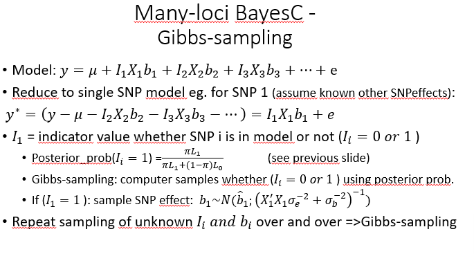
Gibbs-sampling

sample unknown parameters from their posterior distribution

• assuming all already sampled parameters known

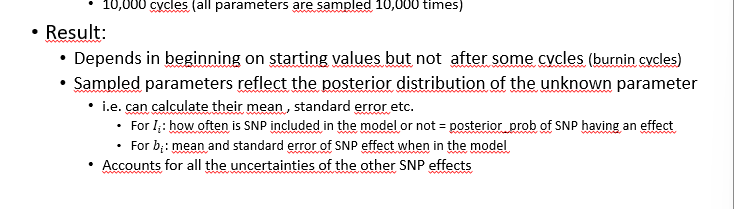
• repeat sampling SNP1, SNP1 … SNP10000, SNP1 etc (10.000 cycles (all parameters are smapled 10.000 times)

result

• depends in beginning on starting values bot not after some cycles (burning cycles)

• sampled parameters reflect the posterior distribtuion of the unknow paramter

• accounts for all the uncertainties of the other SNP effects

BayesC for QTL mapping

plot posterior probability (ii = 1)

or plot variance of local ebv calculate ebv for 250 kb region, calulcate its variance across animals

more clean QTL signals than GWAS

• since model fits all other SNPs, in region, and elseqhere in the genome

  • consider SNP in LD with QTL but not best SNP, GWAS shows LD signal, BayesC: nos ignal (since best SNP is already fitted)

nonlinear methods may be better then GBLUP

GBLUP: unrelaistic assumtion of equal SNP variance

clear benefit in simulation studies, espeically if few genes or if many SNPs are assumed to have zero effect

marginal effect in real data, perhaps true number of genes is large

non-linear statistics is complicated

BayesC uses mixture of normals (not so complicated)

Bayesian methods use .. smapling to fit many SNPs

Gibss

Bayesian methods also useful for QTL mapping

More precise QTL signals