E200 Definitions and Derivations
1/45
There's no tags or description
Looks like no tags are added yet.
Name | Mastery | Learn | Test | Matching | Spaced |
|---|
No study sessions yet.
46 Terms
Convergence back to steady state in the Solow model
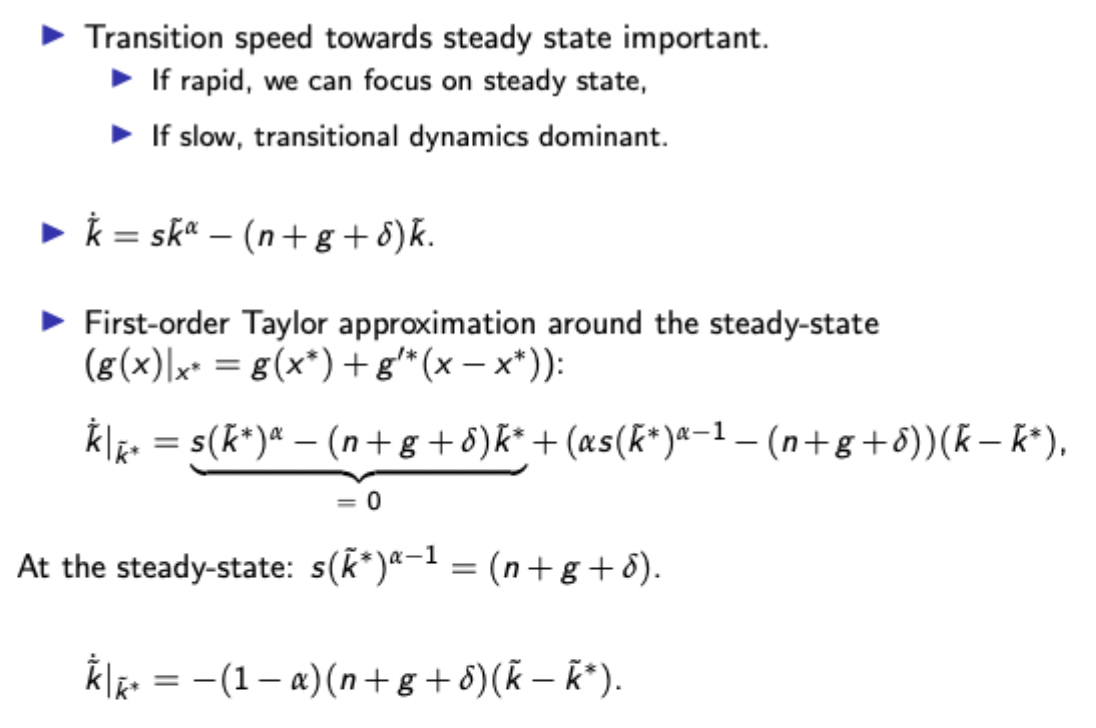
Rate of change in capital per effective worker is clearly increasing in absolute value as it capital per effective worker moves further from the steady state.
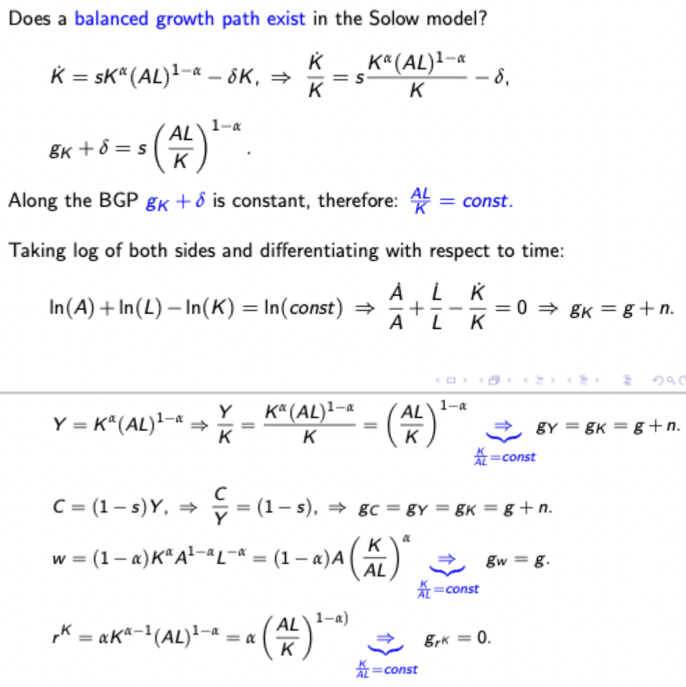
Solow model: growth rates derivations on the balanced growth path
Solow model: golden rule derivation

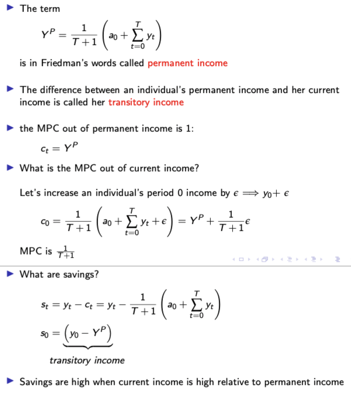
Permanent income hypothesis
Consumption FOC under uncertainty + future consumption as a function of current consumption and shocks to permanent income
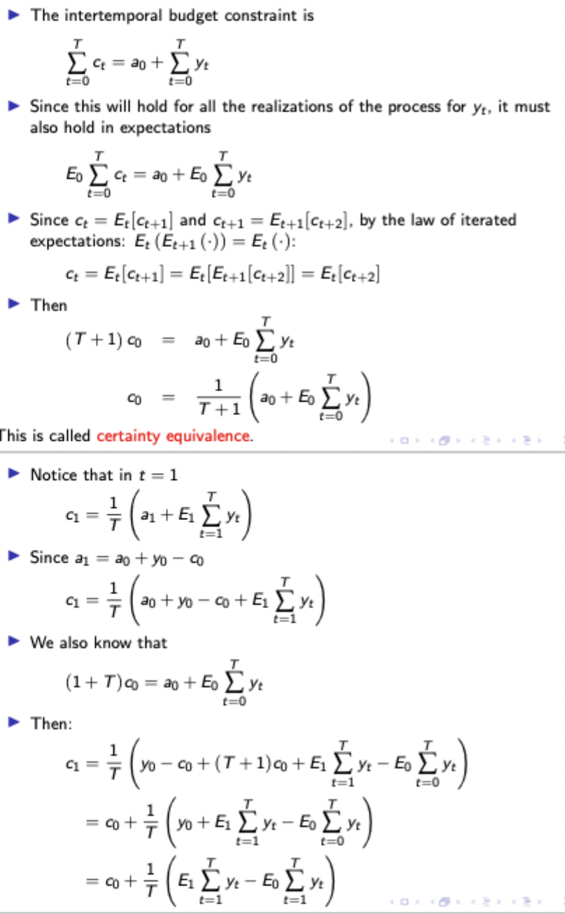
Consumption at t=1 is the same as at t=0, adjusted for unanticipated changes in lifetime income
Whenever you are arguing that a consumer is risk averse, this has to involve discussion of the fact that their utility function is concave in consumption. This can be shown with a graph or just by deriving second derivative as < 0 while the first derivative is > 0. Additionally, for CRRA utility functions, you can wrt. sigma (coefficient) find the derivative of the second derivative wrt consumption to show that the degree of concavity (more / less negative) is increasing wrt. sigma.
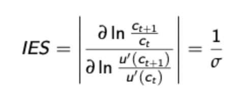
Intertemporal elasticity of substitution
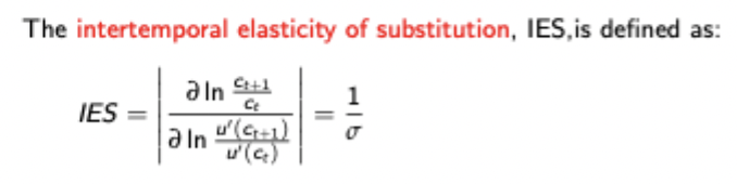
Shows how willing consumers are to substitute consumption across time.
Essentially measures the responsiveness of marginal consumption to changes in the interest rate
Example given above is for CRRA utlity functions
Example of risky assets in consumption under uncertainty

In the general case, high covariance between marginal utility of consumption at t+1 and the return of the asset at t+1 indicates that when consumption at t+1 is low (marginal utility is high), the return will be high, and hence the consumer should buy more of the risky asset as it acts as insurance
Equilibrium conditions in RBC models
Household:
Consumption Euler
Budget constraint
Firm
Profit maximising capital interest and wage rates from production function
Production function
Markets
Y(t) = C(t) + I(t)
I(t) = S(1) = K(t+1) - (1 - depreciation rate)K(t)
Labour supply (determined by labour FOC in consumer’s optimisation problem) = Labour demand (determined by firm’s FOC in profit maximisation problem)
Meaning of shadow price of capital in investment modelling in either form
(when not within the brackets and adjusted by interest rate) this is value at t = 0 of marginally relaxing the BC
(when included in the brackets, hence adjusted by the interest rate and included in the summation) this is the present value (or time = t) value of marginally relaxing the firm’s BC
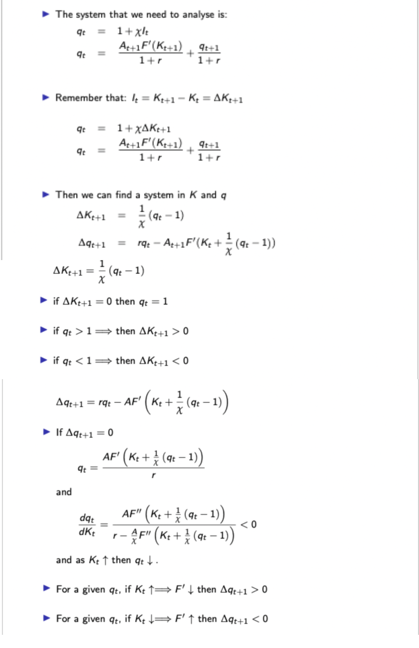
Derivation of phase diagram loci in investment model with adjustment costs
Solow condition for efficiency wages derivation
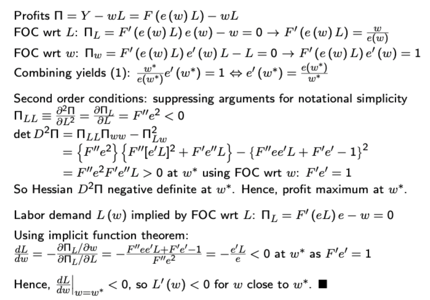
DON’T FORGET TO FIND THE FOC WRT BOTH W AND L. Also include the SOC (hessian) as negative definite to get top marks (include if you have time). Just need to show that the determinant is > 0, and the second derivative wrt labour is < 0.
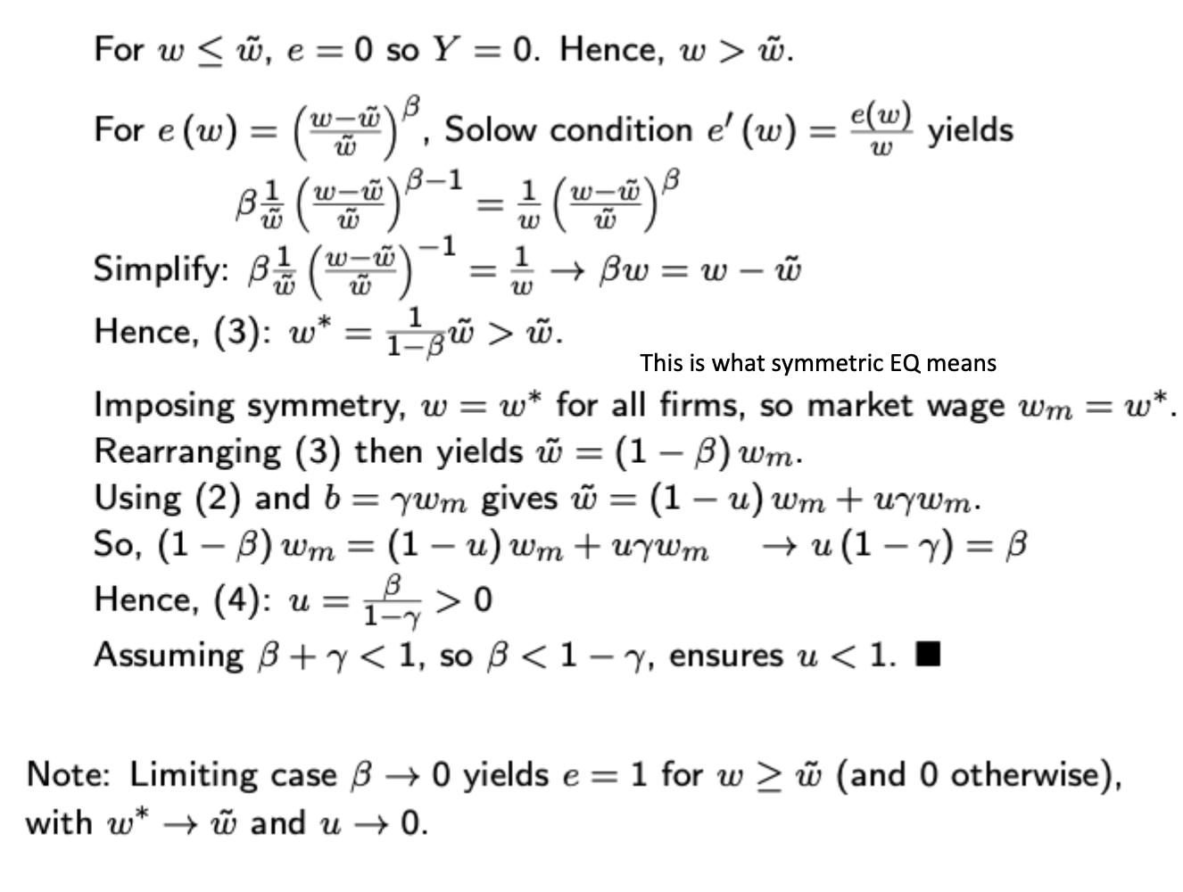
Solow condition with reference wage derivation
Derivation of no shirking condition in Shapiro-Stiglitz model (including labour market steady state)
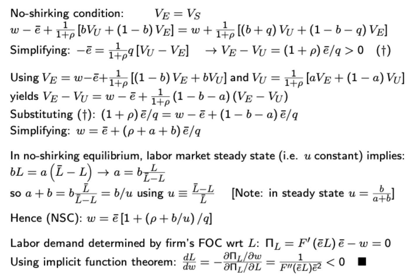
Working out expressions for lifetime utilities for shirkers Vs, employed workers Ve, and unemployed people Vu is simple, though be aware of changes (i.e. adding in unemployment benefits
Key result + derivation in insider - outsider model
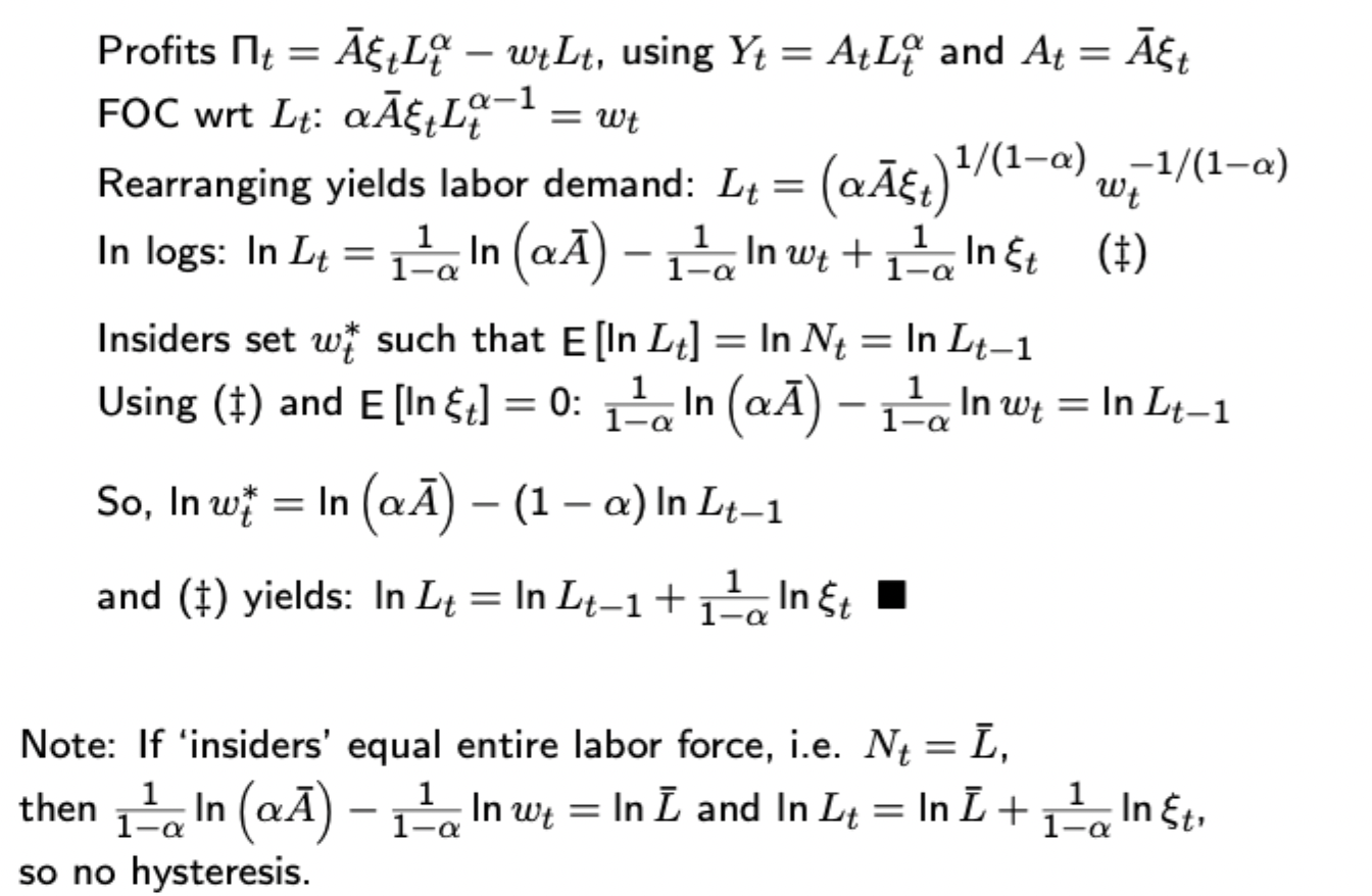
Final result shows how hysteresis can exist due to differences in bargaining power between insiders and outsiders, with log employment following the random walk as shown
Key thing to do is to take logs and expectations to find the optimal wage that will result in expected employment at t being the same as at t-1.
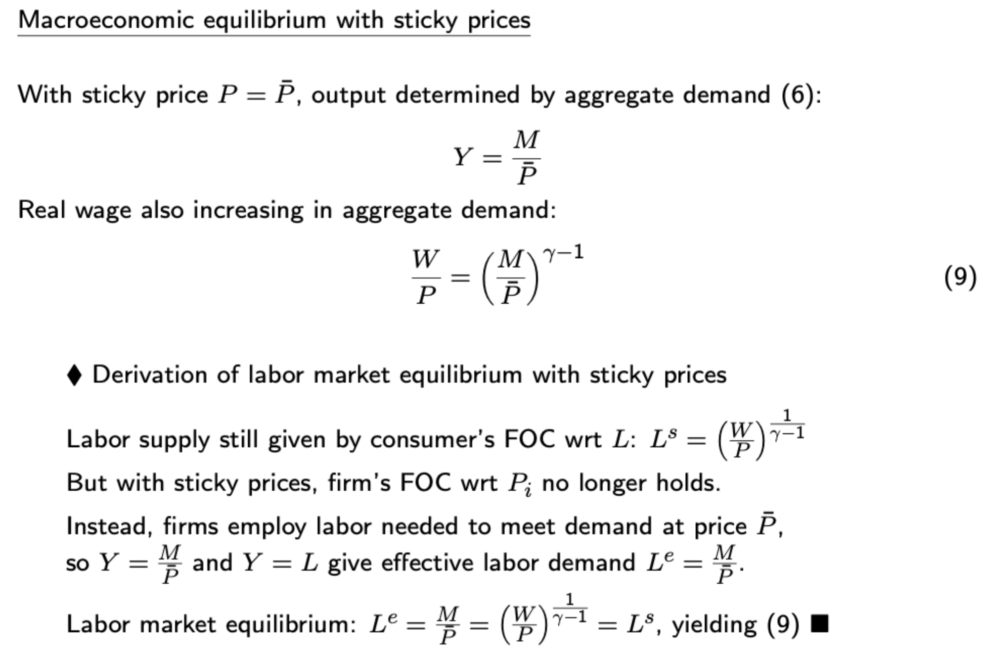
Nominal rigidities: Monopolistic competition model
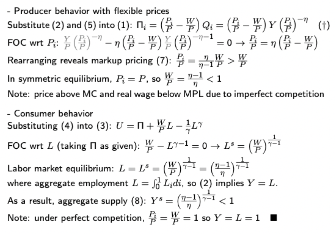
Remember here that when you are solving firm’s pricing problem you are finding the optimal P(i)/P, not the optimal P(i). Also don’t forget that a key part of this is imposing symmetric EQ where P(i) = P
Menu cost model with real rigidities
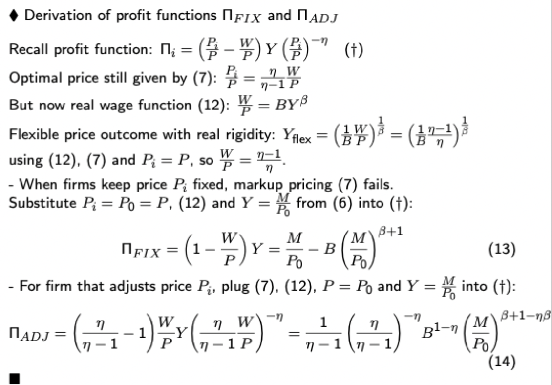
The firm will thus choose the strategy (fix or adjust) that generates the higher payoff, hence this can show how menu costs when there are real rigidities can cause a nash EQ with sticky prices.
Menu cost model without real rigidities - derivation
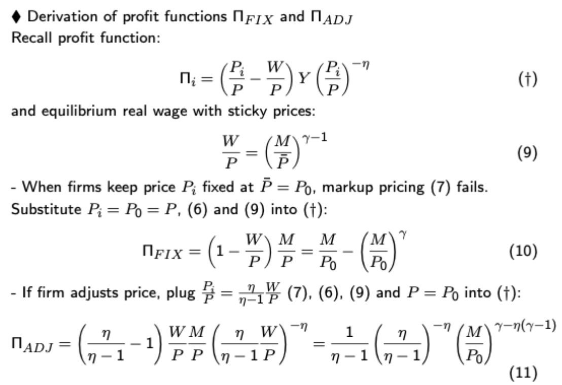
Key point is that you will have derived a real wage function beforehand or be given one, so this part isn’t hard, just sub in the values, ensuring that you remember to plug P=P(0) into the AD function at the end.
Inflation bias - derivation
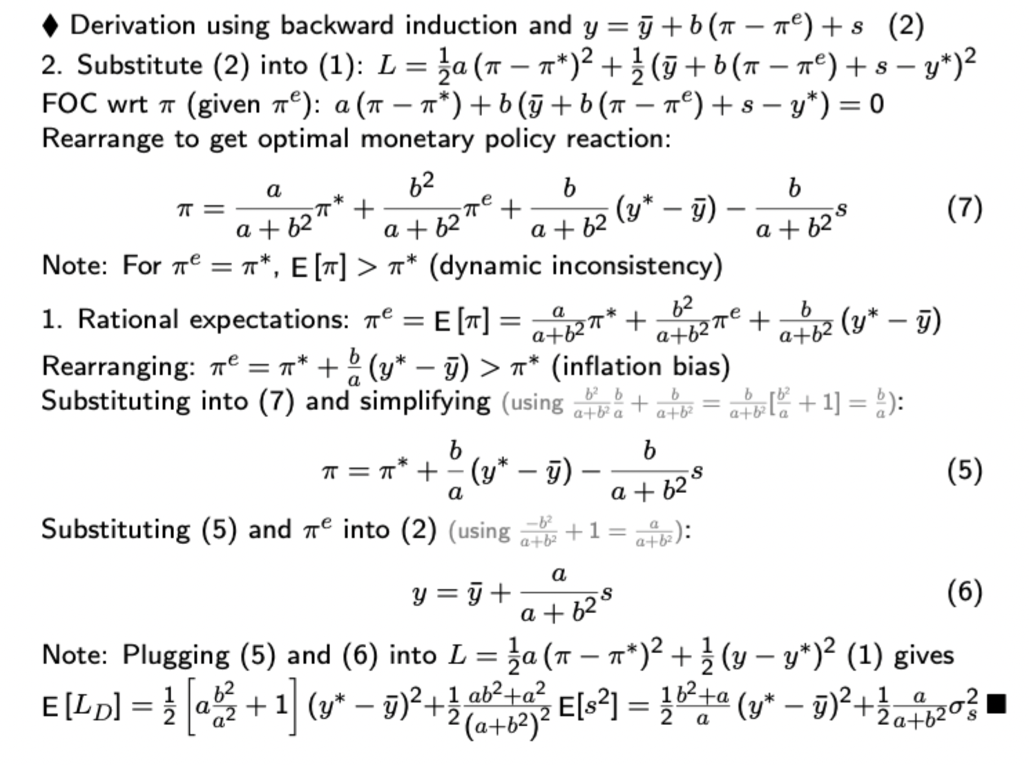
Basic Barro Gordon model: attempts to shift output beyond its natural rate using monetary policy generates an inflation bias due to the public anticipating the policymaker’s attempt to do so.
Solved via backwards induction: public form their inflation expectations by anticipating the policymaker’s objective function.
Backwards looking monetary policy model (Taylor rule derivation)
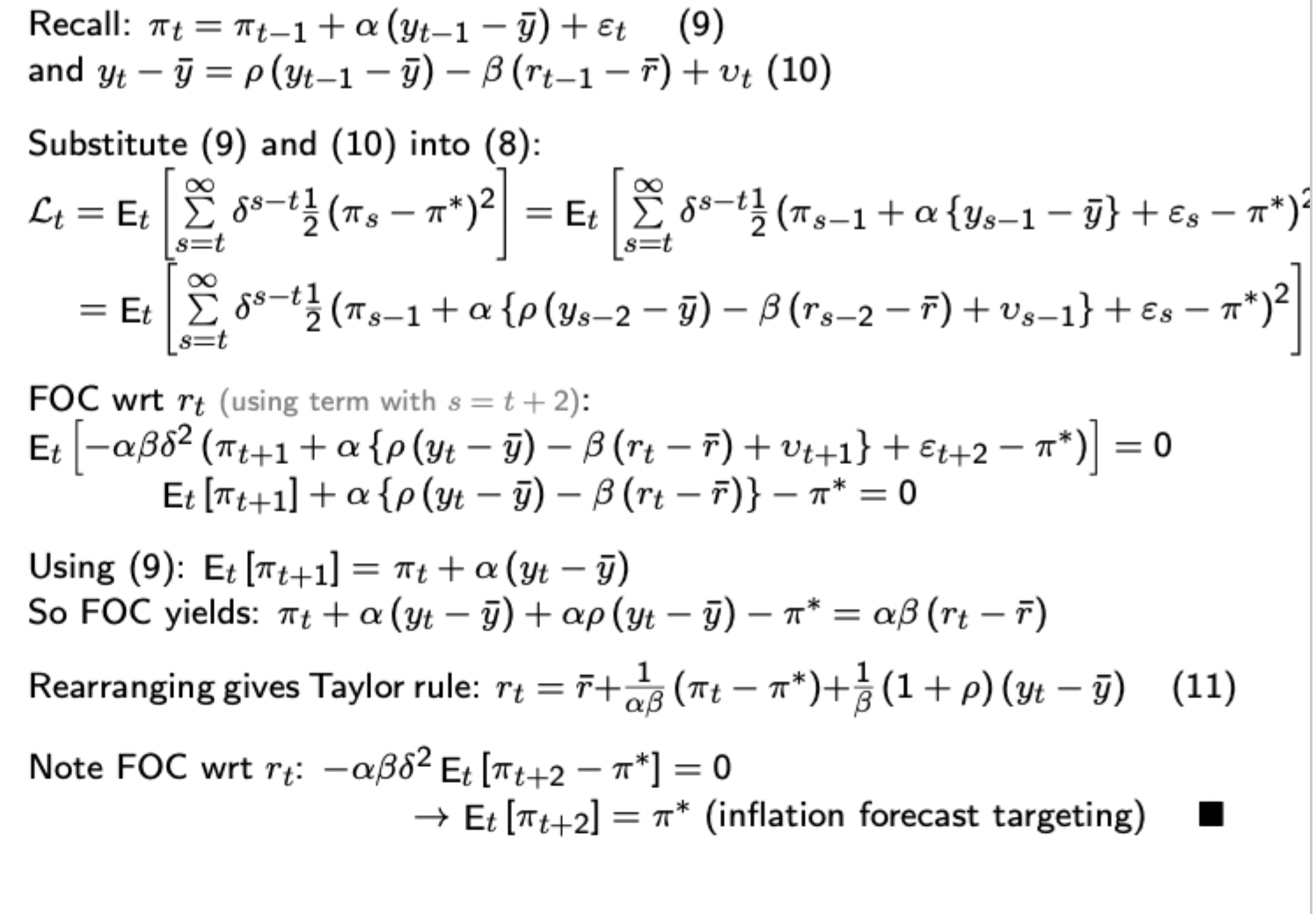
Remember the time period: interest rates set at t affect output at t+1 which affects inflation at t+2
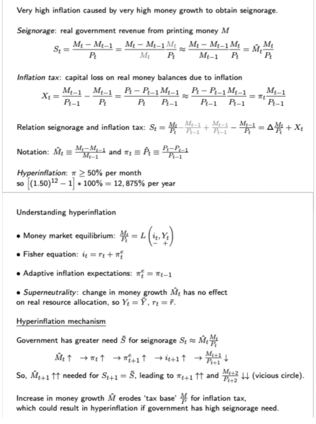
Seignorage + hyperinflation key result and derivation
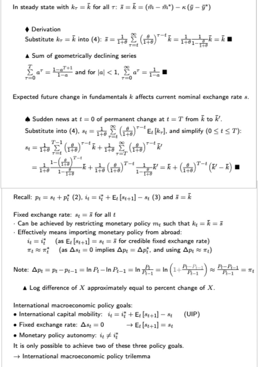
Flexible price monetary model: derivation of nominal exchange rate expression
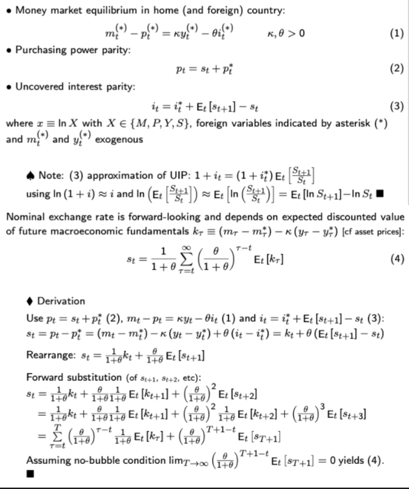
Often questions on this usually require you to show how the e/r reacts to a change in one of the fundamentals (can be immediate / anticipated, and temporary / permanent). The best way to show this is to mark the expected fundamentals with the change as E[k’], find E[k’] - E[k], then use this in the summation sign to find s’ - s.
Also explicitly state the no bubble condition. This can sometimes help to illustrate if you have done some addition wrong. Also if the fundamentals change more than once, you need to account for how the exchange rate changes every time (i.e. if output falls by 10% at t then 2% at t+1 before staying at that level from then on, you will have an initial drop at t, then an adjustment at t+1 before it levels off).
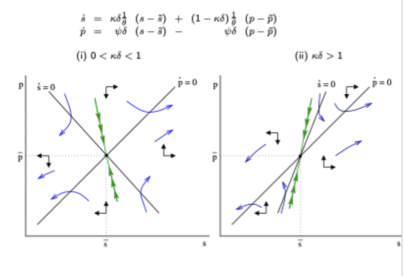
Dornbusch derivation
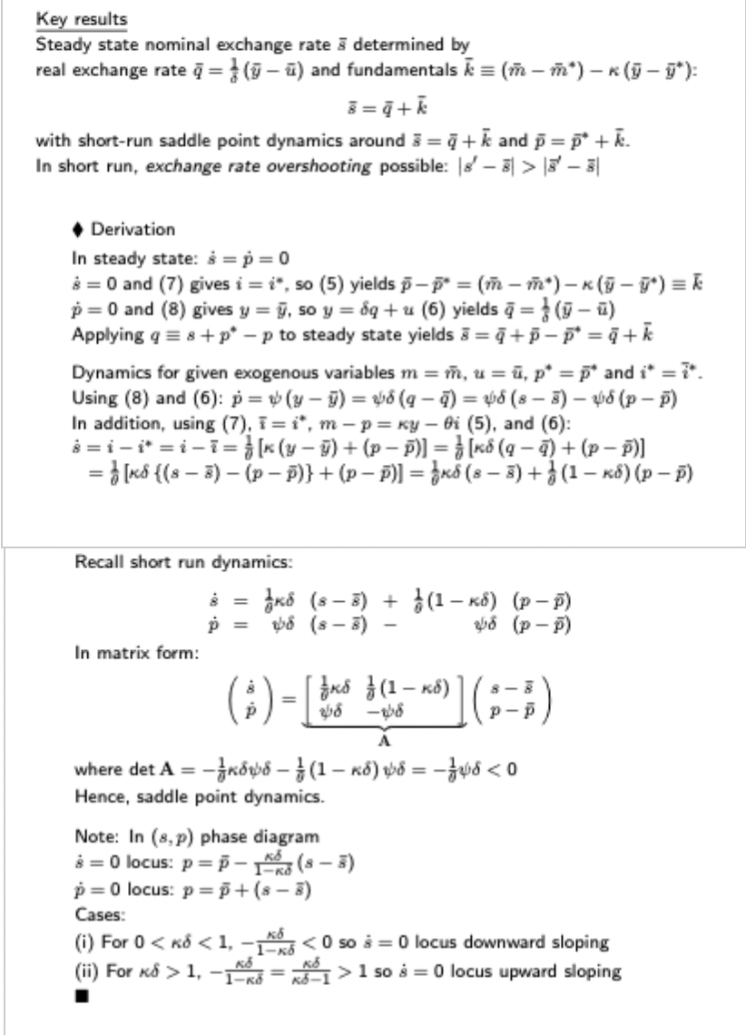
The equations you are given to start with are money market EQ, open economy IS equation, UIP with perfect foresight and a predetermined price (no jumps) with price adjustment Philips Curve.
Dornbusch - overshooting / undershooting / neither result
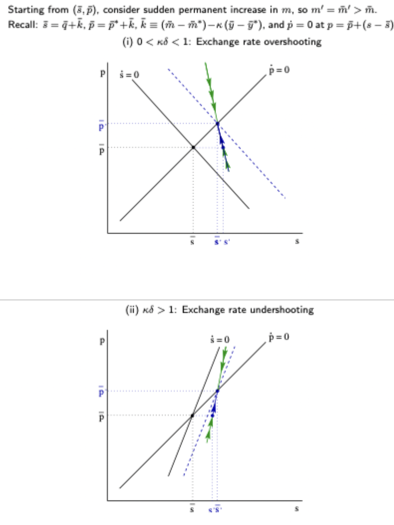
Also see revision class slides for the effect of a temporary shock
Harrod Balasa Samuelson: key result and derivation
Key result: countries with higher productivity in tradables compared to non-tradables tend to have a higher aggregate price level
See slides for derivation (too long for a flashcard)
Ricardian Equivalence derivation
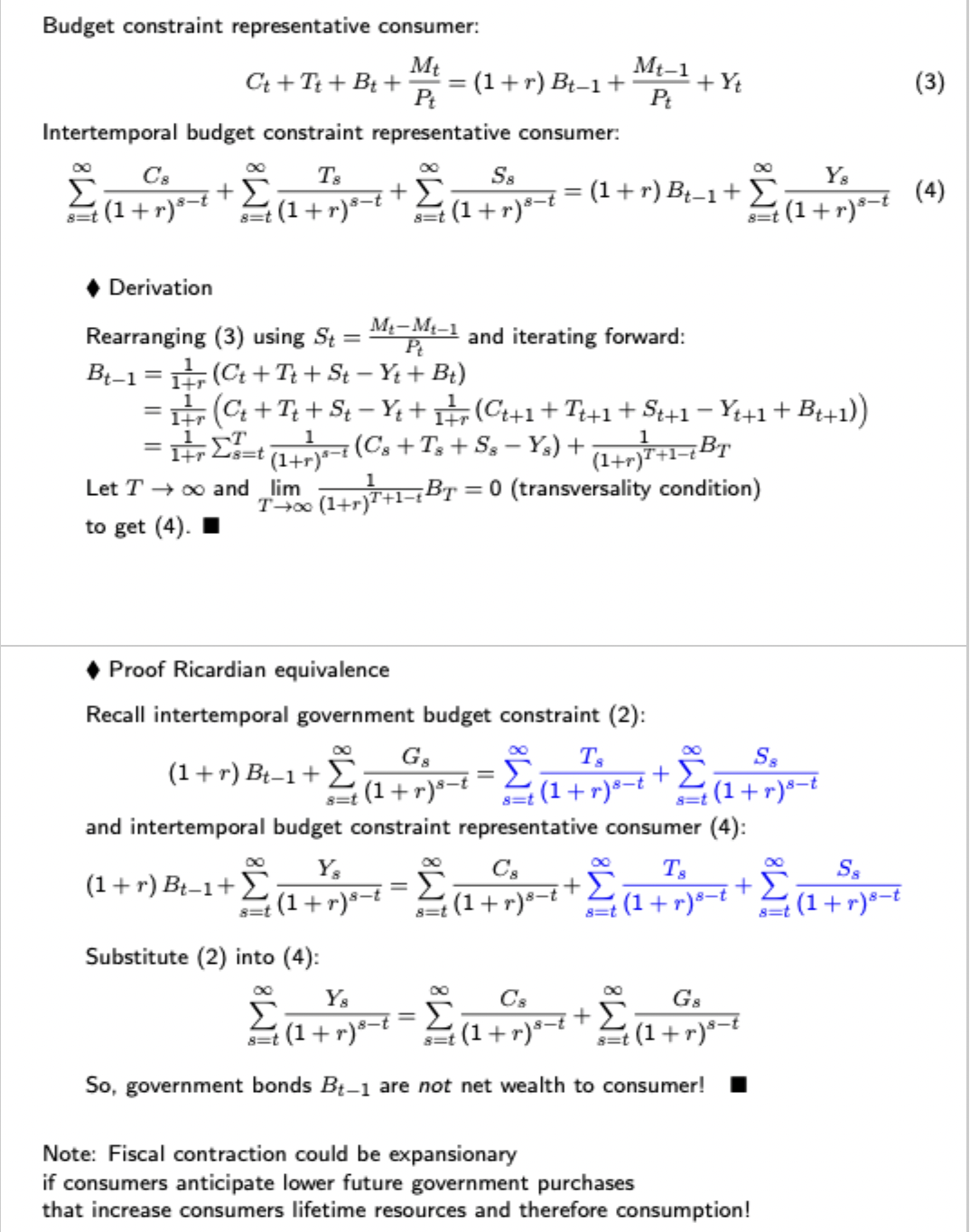
I.e. how the government finances its expenditure (tax vs bond) has no aggregate effect
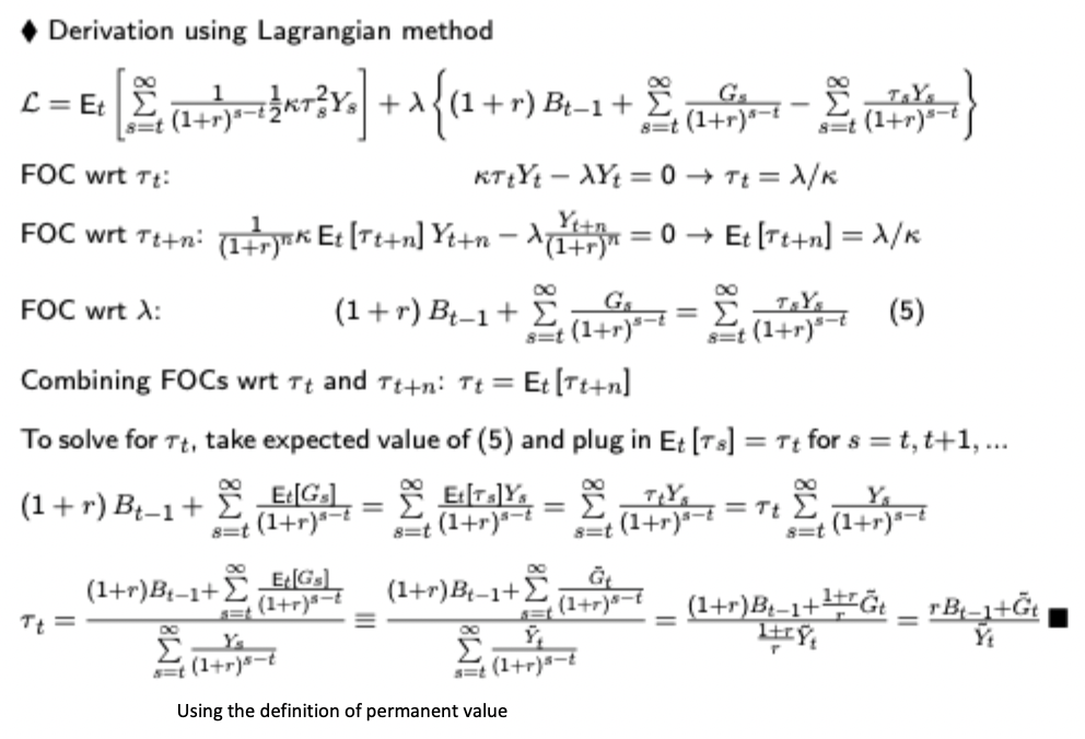
Tax smoothing model derivation
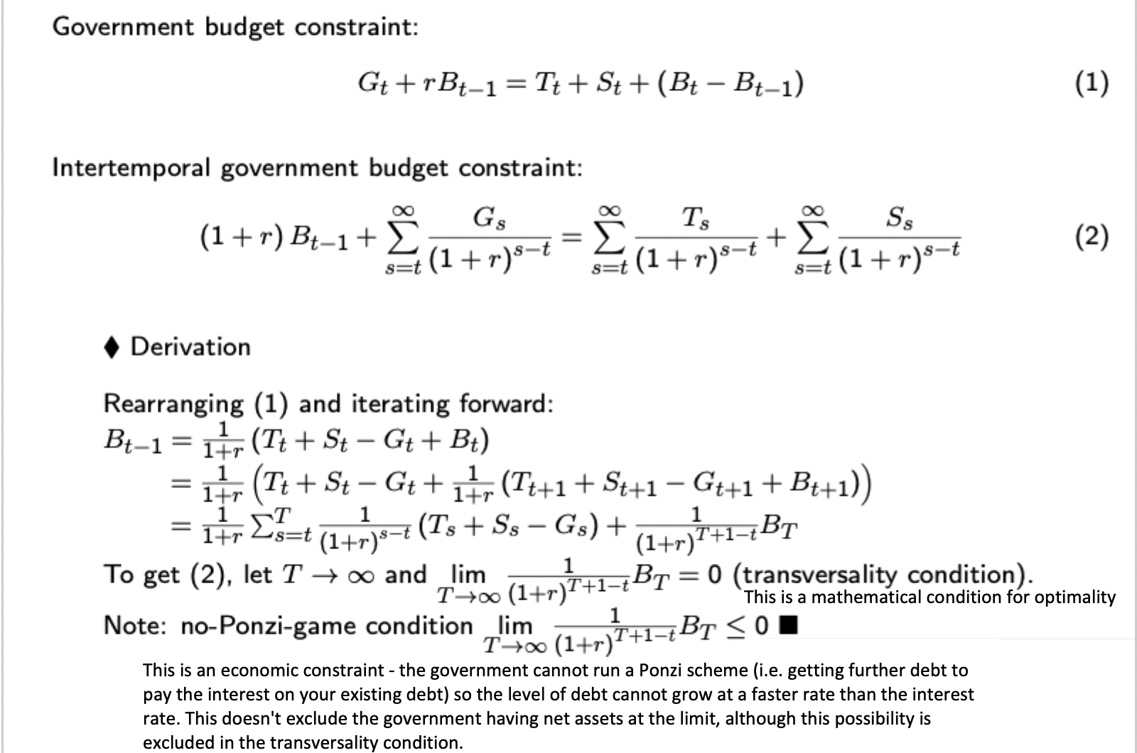
No Ponzi condition meaning in fiscal policy
Government cannot run a ponzi scheme - the present value of government borrowing as T goes to infinity must be less than or equal to 0 indicating that the government cannot continually borrow to finance debt servicing without repayment.
Inada conditions + meaning
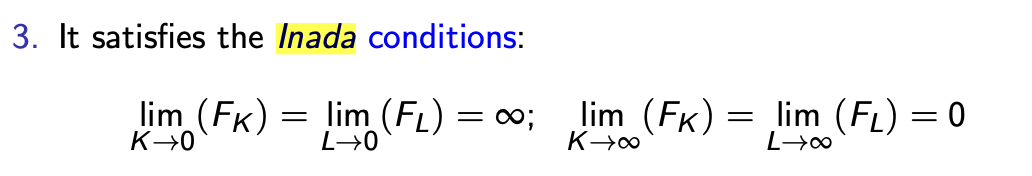
Example given for base Solow model production function. When combined with concavity of the production function, they guarantee stability and the existence and uniqueness of a steady state equilibrium
Gov’t budget deficit ratio in tax smoothing model
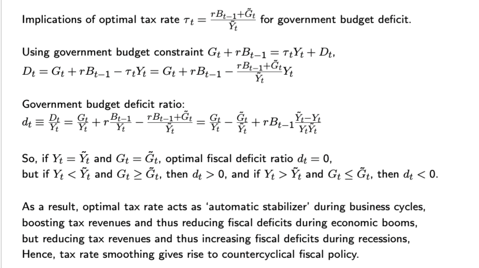
Tax smoothing - effect of a temporary rise in G
Tax: immediate and permanent tax hike. Permanently higher because the lifetime DWL from raising the requisite revenue are minimised by the tax smoothing result
Deficit: Temporary rise in spending, during which taxes are permanently raised so the change in tax is smaller than the change in spend. The government thus funds the spending in part by increased borrowing keeping the deficit constant until the increase ends. After that, it runs a permanent surplus due to higher tax revenues at the old spending level. This is sufficient to service its debt.
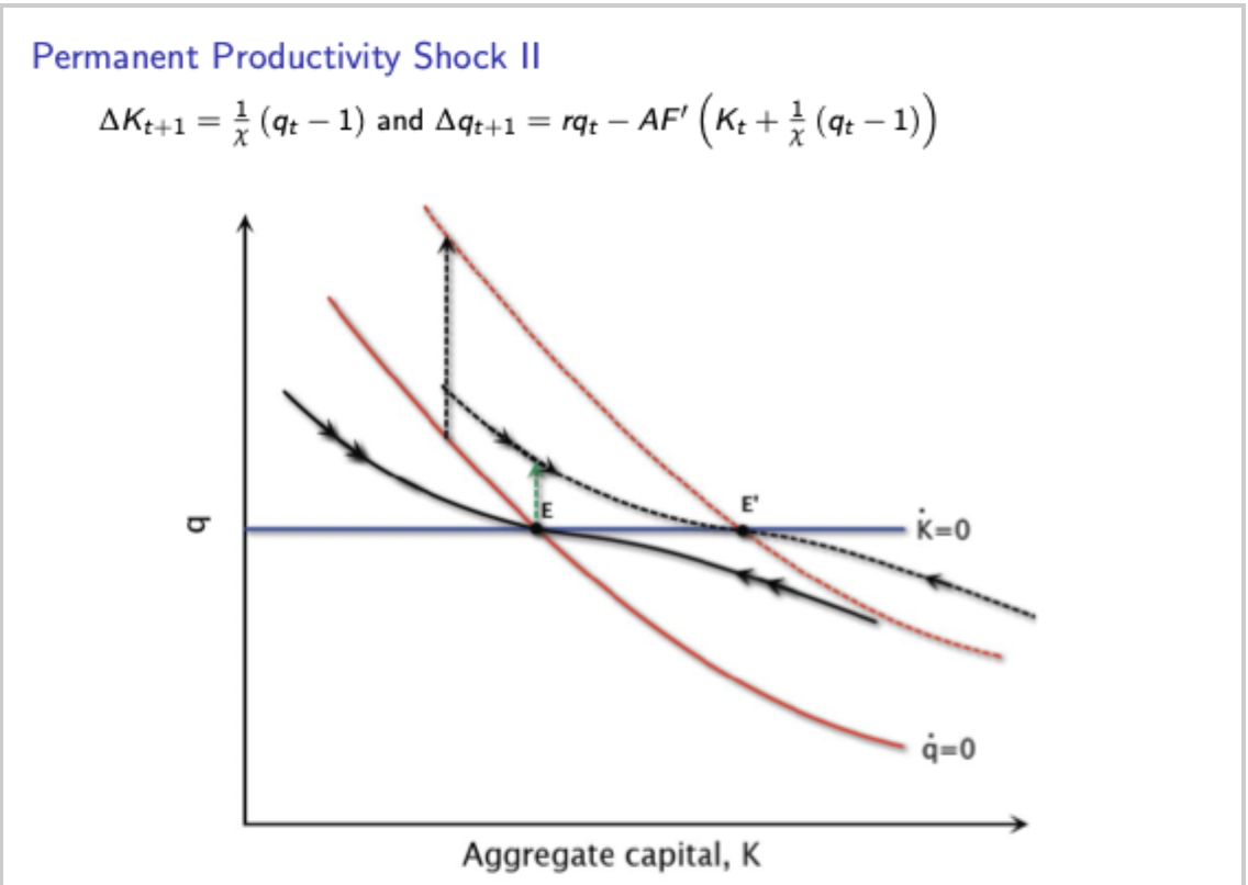
Investment model: Phase diagram after permanent productivity shock
Investment model: Phase diagram with temporary shock
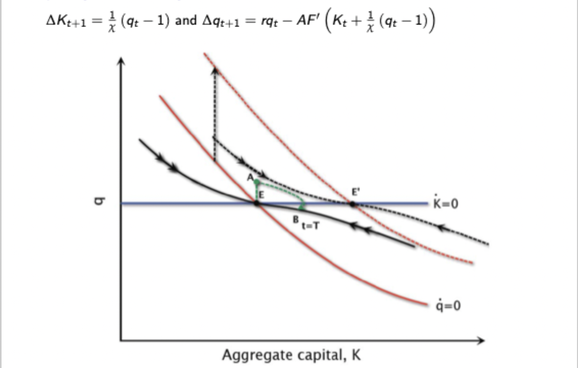
Smaller jump, since increase in infinite time marginal product is smaller for a temporary shock. Then producers understand that when the shock expires at t = T, you have to be back on the original saddle path.
The locus shifts. The change in productivity affects present value of profits and marginal product of capital, so while K does not change immediately, the jump in q(t) makes it optimal to invest / disinvest, reducing K(t+1). Changing the capital stock changes the marginal product of capital, affecting q(t+1), so the new investment / disinvestment declines over time. Eventually q will move to being > (or <) 1 again, making it optimal for firms to invest (disinvest) gradually (due to investment adjustment costs) to prepare for the change in productivity back to the original level. Once this happens it transitions smoothly back onto the original saddle path moving back towards the original steady state.
Without adjustment costs, the firm would move straight onto the new saddle path and stay there until it had to move back onto the old saddle path (big jump in its capital stock).
Monopolistic competition model: effects of a change in AD with sticky vs flexible prices
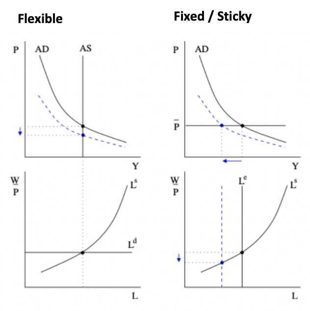
Sticky prices mean AD (Y = M/P where P is fixed) is the determinant of output, flexible prices mean AS is the determinant of output.
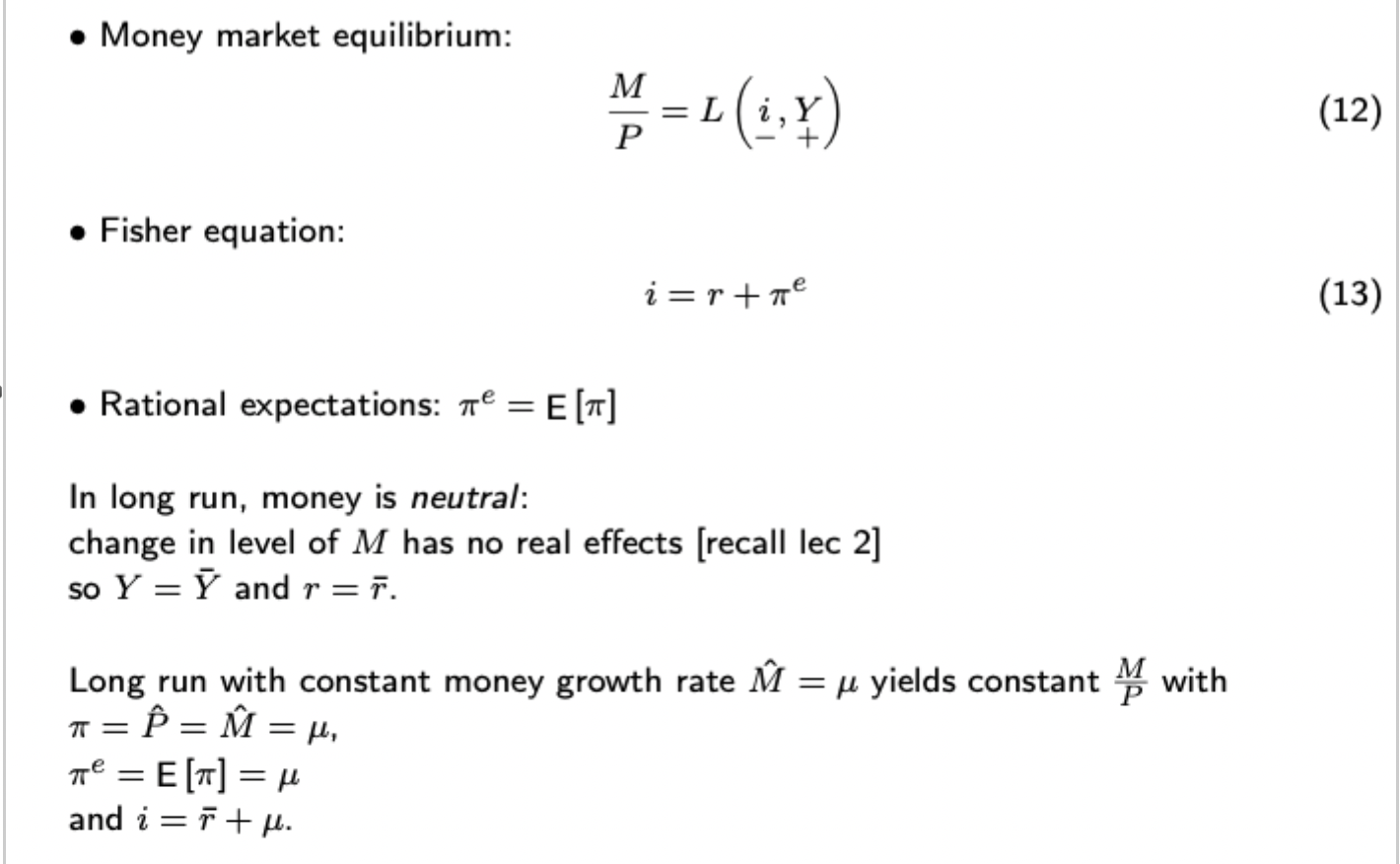
Explanation of long run monetary neutrality
Flexible price monetary model: derivation of macroeconomic policy trilemma using steady state expression of forward looking nominal exchange rates
Dornbusch basic dynamics
Government intertemporal budget constraint derivation
Intuitions for the mechanism through which a fall in future expected aggregate output can impact the exchange rate
Money market EQ: a fall in (log) output will reduce transactions demand for money. This causes households’ real money balances to rise relative to demand, and so have excess real money balances that they use to buy more goods, hence raising the prices to restore the money market EQ.
Purchasing power parity: A rise in Britain’s prices makes it less competitive, reducing demand for its currency and raising its price of foreign currency (i.e. depreciating the exchange rate)
Uncovered interest rate parity: A depreciation of the exchange rate is now expected, which makes it less attractive to invest in Britain’s deposits / bonds, reducing current demand for Britain’s currency, and hence leading to an immediate depreciation.
Method of finding the equilibria in the monopolistic competition model (flexible prices and perfect competition in the labour mrarket)
Solve the firm’s profit maximisation problem to determine its markup pricing P(i)/P above MC and its markdown pricing of real wage W/P below MPL
Solve utilmax problem for consumer to determine optimal labour supply then combine with labour demand from firm’s problem
Use this to show that aggregate output is determined by aggregate supply
Permanent value of a variable (specifically useful in the tax smoothing model)
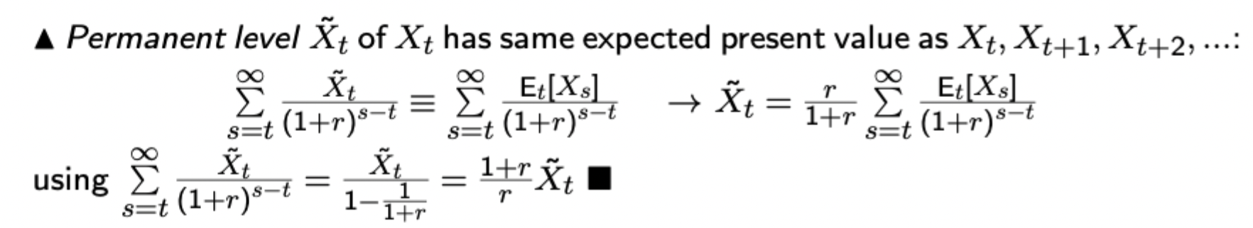
Important geometric sum concepts to remember
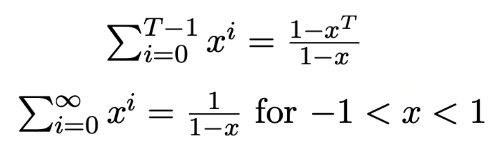
Most useful in tax smoothing model. You know the bottom one well but note also that the top expression holds for all values of x.
Solow model: analysing growth rates of capital per effective labour
The growth rate depends on the distance away from the steady state (which you know how to calculate).
When doing growth rate comparisons, always see if you can find the distance from the steady state as a means of finding out which has a higher growth rate of capital per effective labour.
Relationship between relative risk aversion and the intertemporal elasticity of substitution with CRRA utility
The IES is the inverse of the coefficient of relative risk aversion. This implies that high risk aversion implies an unwillingness to change your consumption profile over time (this indicates a greater level of consumption smoothing).
This relationship is arbitrary - being afraid of gambles and being unhappy about variation in a deterministic consumption paths are not equivalent concepts, so should be captured by separate parameters, however this is a feature of the the CRRA utility function.
Dealing with consumption questions with interest rates and savings
The standard ‘permanent income’ approach with a constant interest rate would imply that, sparing the possibility of very high beta and r, the consumer would borrow immensely to consume income in period 0.
Therefore, most questions on this will not want you to solve for optimal c(0) using the present value budget constraint, rather they play around with the income stream and often include variable interest rates that can’t be taken out of the summation.
Investment: why is investment positive when q>1
A marginal additional unit of capital (i.e. the shadow price - relaxing the budget constraint etc.) offers a value of q, whereas the ‘direct cost’ of investing is 1 (K(t) = I(t) - K(t+1) an additional unit of capital ‘costs’ 1. How strongly the firm responds to the gap between q and 1 depends on the adjustment costs, the higher the adjustment costs on the margin (shown by chi), the smaller the response to the given gap.
Re the stock market valuation, if there are constant returns in production and investment technology, marginal q (that we find) and average q (more closely resembling Tobin’s q (ratio of market value of firm’s capital to replacement cost of this capital)) align and a ‘stock market valuation’ can be found. q in this case is a lagrange multiplier, not intended as a stock market valuation, and a stock market would also value far more than just what is represented by average q (risk premia, subjectivity in valuations, etc.)
Monopolistic Competition: Sticky Prices