MEC320 Tutorial 3 Numerical Methods

Why do we need to discretize PDEs? What is the difference between a continuous function/equation and a discretized one?

Discretization transforms continuous PDEs into algebraic equations that can be solved numerically. A continuous function is defined over a continuum, while a discretized one is defined only at discrete points.

   Why do we talk about approximation in the context of discretization and what is the truncation error?

Discretization approximates derivatives, and truncation error is the difference between the true derivative and its numerical approximation.

What do we mean by the order of accuracy?

The order of accuracy defines how the error reduces as the mesh is refined. Higher-order schemes decrease error faster.

Why is interpolation needed in the context of the FVM?

In FVM, values are known at cell centers, but fluxes are needed at faces—interpolation estimates these values.

What is the advantage of the 1^st order upwind scheme?

It is stable and ensures boundedness by using upstream values, though it is only first-order accurate.

What does the ‘boundedness’ refer to in the context of convection schemes?

Boundedness ensures that the numerical solution stays within physical limits, avoiding overshoots or undershoots.

What can you do to improve the accuracy of a CFD simulation from numerical point of view?

Refine the mesh, use higher-order schemes, improve boundary conditions, and reduce the time step if needed.

Compare finite difference and finite volume methods, and discuss the advantages and disadvantages of each of these methods.

• FDM: Easy to implement on structured grids but not conservative.

• FVM: Conservative and suitable for complex geometries; handles unstructured meshes.

Consider the following stencil.

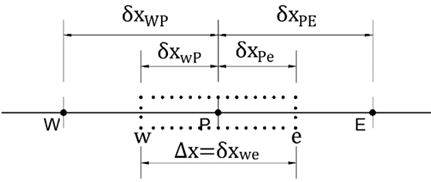
The discretised for of … using the central differencing scheme is

\displaystyle \left(\frac{d\phi}{dx}\right)w

\displaystyle \frac{\phi_P - \phi_W}{\delta x{WP}}

Discretise … on a uniform mesh using central difference FV method

\displaystyle k \frac{d^2 T}{dx^2}

\displaystyle \frac{k}{\Delta x^2} T_W + \frac{k}{\Delta x^2} T_E - \frac{2k}{\Delta x^2} T_P

Discretise … , where rho and U are const. and I > 0 on a uniform mesh using:

a) 1st order upwind

b) central difference FV methods

\displaystyle k \frac{d^2 T}{dx^2}

\displaystyle \frac{k}{\Delta x^2} T_W + \frac{k}{\Delta x^2} T_E - \frac{2k}{\Delta x^2} T_P

Discretise … where rho and U are const. on a uniform mesh using a) 1st order upwind b) Central Diff FVM

\displaystyle \frac{d}{dx}(\rho U \phi)

a)\displaystyle\frac{\rho U (\phi_P - \phi_W)}{\Delta x}

b)\displaystyle\frac{\rho U (\phi_E - \phi_W)}{2 \Delta x}

What are the differences between implicit and explicit discretization methods? What are the pros and cons of each method?

• Explicit: Solves directly using current values.
   • Pros: Simple, fast per time step
   • Cons: Conditionally stable, requires small time steps

• Implicit: Solves using future time values (requires system solving).
   • Pros: Unconditionally stable
   • Cons: More complex and computationally expensive

Which one (implicit or explicit) can be more unstable computationally? Why?

Explicit methods can be unstable if the time step is too large, violating the CFL condition.

Which one (implicit or explicit) provides more flexibility on the choice of the time step and how can this be an advantage?

Implicit methods allow larger time steps without violating stability constraints, making them better for stiff or steady problems.

Explain why when the mesh is refined, often the time step also needs to be reduced?

Because the stability condition (e.g., CFL) depends on cell size:

\displaystyle \Delta t \leq \frac{\Delta x}{U}

refining the mesh smaller dx requires smaller dt for stability

What is CFL? What is the general requirement on this value?

The Courant–Friedrichs–Lewy (CFL) number determines the maximum stable time step for explicit schemes.

CFL=\frac{U\Delta x}{\Delta t}

For stability in explicit schemes:

\displaystyle \text{CFL} \leq 1

What is the pressure-velocity coupling problem? What are the methods available to this problem?

In incompressible flows, pressure and velocity are interdependent, but pressure doesn’t have its own equation. Methods to handle this include:

• SIMPLE

• SIMPLER

• PISO

• Coupled solvers

What are the differences between density-based and pressure-based solvers?

• Density-based: Suitable for compressible flows; solves continuity using density changes.

• Pressure-based: Suitable for incompressible flows; solves pressure-velocity coupling using correction algorithms (e.g. SIMPLE).

Describe the SIMPLE procedure – in terms of the main procedures.

• Guess pressure field

• Solve momentum equations

• Compute pressure correction

• Update pressure and velocity

• Iterate until convergence

What do we mean by ‘pressure correction’? How is continuity achieved in SIMPLE scheme?

Pressure correction is a change applied to the guessed pressure to enforce mass conservation. Continuity is achieved by ensuring divergence of the corrected velocity is zero.

How to solve the linearised algebraic equations in CFD? Why are iterations needed even though the equations are linearised?

• Solve using iterative methods (e.g. Gauss-Seidel, TDMA)

• Iterations are needed due to equation coupling and non-linearity in the overall system.

In pressure-based solutions, there are segregated and coupled algorithms. Describe each method. Discuss pros and cons for each method.

• Segregated: Solves equations one at a time; more stable but slower.

• Coupled: Solves momentum and pressure equations simultaneously; faster but requires more memory.

What are the main differences between direct and iterative methods? Their advantages and disadvantages?

• Direct: Solve equations exactly (e.g. LU decomposition); fast for small problems but memory-heavy.

• Iterative: Approximate solution via successive steps (e.g. Gauss-Seidel); scalable and memory-efficient.

What is the under-relaxation factor? Why is this necessary in CFD?

It slows the rate of variable update per iteration:

\displaystyle \phi_{\text{new}} = \phi_{\text{old}} + \alpha (\phi_{\text{computed}} - \phi_{\text{old}})

Used to stabilize convergence.

\displaystyle 0 < \alpha < 1

Is the energy equation solved together (coupled) with the momentum equations in segregated, coupled or density based algorithm?

• In coupled and density-based solvers: yes

• In segregated solvers: not necessarily — can be solved separately if thermal effects are weak.

Are turbulence models solved together with momentum equations in any algorithms?

No, turbulence models are solved separately but influence the momentum equations via modeled Reynolds stresses.

In pressure-based algorithms, there is a step ‘update mass flux’ – what does this do?

It recalculates face fluxes based on the corrected pressure and velocity fields to ensure conservation of mass.

For the flow over an aeroplane with the highest Mach number around 0.8. What solver would you choose to use – density or pressure based and why?

Use a density-based solver, since the flow is compressible and near-transonic.

The RANS equations are non-linear and coupled. What do we mean by non-linear? And coupled?

• Non-linear: Equations include products of variables (e.g. $\displaystyle u \frac{\partial u}{\partial x}$)

• Coupled: Variables depend on each other and must be solved simultaneously.

The convergence in Gauss-Seidel iteration is often slow. Explain why? How to overcome this? How does multigrid method work?

• Slow because it reduces high-frequency error first

• Use multigrid, which solves on coarser grids to eliminate low-frequency errors, then refines solution on finer grids

In what applications would you use structured mesh approaches? Why?

Structured meshes are used for simple geometries (e.g. pipes, channels). They offer:

• Easier implementation

• Faster solvers

• Better control over grid resolution

In what applications would you use unstructured mesh approaches? Why?

Unstructured meshes are used for complex geometries (e.g. airfoils, combustion chambers). They offer:

• Greater flexibility in meshing irregular domains

• Local refinement without excessive node count

Why is it always useful to try to use structured mesh near the wall?

Structured meshes allow better control of wall-normal spacing, which is essential for resolving boundary layers and meeting y+ criteria.

How would you measure mesh quality?

Using metrics such as:

• Skewness

• Aspect ratio

• Orthogonality

• Smoothness of cell size transitions

Is it sensible to use high aspect ratio grid elements/cells in regions where flow is developing? Why?

No — in developing flow, gradients exist in multiple directions. High aspect ratio cells may not capture transverse variations accurately and can degrade solution quality.

What is the aim of a mesh independence study?

To ensure the solution does not significantly change with further mesh refinement. Confirms that numerical error due to mesh is negligible.

What are the meshing rules for wall-function turbulence model?

• First cell center should be in the log-law region: 30 < y+ < 300

• Avoid high skewness or abrupt transitions in cell size near walls.

What considerations would you give to generate a mesh for a turbulent boundary layer with a resolved turbulence model?

• Place first cell at y+ <1

• Use fine wall-normal spacing

• Apply smooth grid growth (e.g. geometric stretching < 1.2)

What is residual?

A residual is the imbalance or error in the discretized equation at each iteration. It measures how far the current solution is from satisfying the equation.

What is the difference between the scaled and normalised residuals?

• Scaled residuals: Raw or dimensional values

• Normalised residuals: Residuals divided by a reference (e.g. initial value), enabling comparison across cases or variables

What are the differences between the residual at one node and an ‘overall’ residual for all grids?

• Node residual: Local error at a specific point

• Overall residual: Aggregated error across the entire domain (e.g. L2 norm)

What factors will you check if the convergence of your simulation is slow (or even diverging)?

• Mesh quality (skewness, aspect ratio)

• Under-relaxation factors

• Boundary conditions

• Initial guess

• Time step (for transient)

• Solver settings

What is the benefit of using monitoring points for the solution of certain flow variables?

They help track physical convergence (e.g. pressure, velocity at key locations), which is often more meaningful than just checking residuals.

What is verification? What is validation? What are the differences between the two?

• Verification: Ensures the equations are solved correctly (math is right)

• Validation: Ensures the correct equations are being solved (model represents reality)
  Difference:

• Verification answers: "Did we solve the equations right?"

• Validation answers: "Did we solve the right equations?"