Algorithms & Data Structures Cartes | Quizlet

Greedy Algorithm

an algorithm that follows problem solving heuristic of making optimal choices at each stage. Hopefully finds the global optimum. An example would be Kruskal's algorithm.

Divide and Conquer

works by recursively breaking down a problem into two or more sub problems until the problems become simple enough to be solved directly. An example would be mergesort.

Recursive Algorithms

solve a problem by solving smaller internal instances of a problem -- work towards a base case.

Dynamic Programming

Break down a problem into smaller and smaller subproblems. At their lowest levels, the subproblems are solved and their answers stored in memory. These saved answers are used again with other larger (sub)problems which may call for a recomputation of the same information for their own answer. Reusing the stored answers allows for optimization by combining the answers of previously solved subproblems.

Selection Sort

Non-stable, in place sort. Has an N-squared order of growth, needs only one spot of extra space. Works by searching the entire array for the smallest item, then exchanging it with the first item in the array. Repeats this process down the entire array until it is sorted.

Insertion Sort

Stable, in place sort with an order of growth which is between N and N-squared, needs only one spot of extra space and is dependent on the order of the items. Works by scanning over the list, then inserting the current item to the front of the list where it would fit sequentially. All the items to the left of the list will be sorted, but may not be in their final place as the larger items are continuously pushed back to make room for smaller items if necessary.

ShellSort

Non-stable, in place sort with an order of growth which is undetermined, though usually given at being N-to-the 6/5. Needs only one spot of extra space. Works as an extension of insertion sort. It gains speed by allowing exchanges of entries which are far apart, producing partially sorted arrays which are eventually sorted quickly at the end with an insertion sort. The idea is to rearrange the array so that every h-th entry yields a sorted sequence. The array is h-sorted.

Quick Sort

Non-stable, in place sort with an order of growth of NlogN. Needs lgN of extra space. It has a probabilistic guarantee. Works by making use of a divide and conquer method. The array is divided into two parts, and then the parts are sorted independently. An arbitrary value is chosen as the partition. Afterwards, all items which are larger than this value go to the right of it, and all items which are less than this value go to the left of it.

We arbitrarily choose a[lo] as a partitioning item. Then we scan from the left end of the array one by one until we find an entry that is greater than a[lo]. At the same time, we are scanning from a[lo] to the right to find an entry that is less than or equal to a[lo]. Once we find these two values, we swap them.

3-Way Quick Sort

Non-stable, in place sort with an order of growth between N and NlogN. Needs lgN of extra space. Is probabilistic and dependent on the distribution of input keys.

Mergesort

Stable sort which is not in place. It has an order of growth of NlogN and requires N amount of extra space. Works by dividing an array in half continuously into smaller and smaller arrays. At the lowest level, these arrays are sorted and then merged together after sorting in the reverse order they were divided apart in.

Heap Sort

Non-stable, in place sort which has an order of growth of NlogN. Requires only one spot of extra space. Works like an improved version of selection sort. It divides its input into a sorted and unsorted region, and iteratively shrinks the unsorted region by extracting the smallest element and moving it into the sorted region. It will make use of a heap structure instead of a linear time search to find the minimum.

Lower Bound on the complexity of pairwise comparisons

No compare based sorting algorithm can have fewer than ~NlogN compares

Counting Sort (Key Indexed sort)

An integer sorting algorithm which counts the number of objects that have a distinct key value, and then used arithmetic on those countes to determine the positions of each key value in the output array.

It cannot handle large keys efficiently, and is often used as a subroutine for other sorting algorithms such as radix sort.

Has a time complexity of N.

LSD Radix Sort

Stable sort which sorts fixed length strings. Uses an axillary array, and therefore is not in place. Goes through to the last character of a string (its least significant digit), and takes its value. All strings given are then organized based on the value of their least significant digit.

Following this, the algorithm proceeds to the next least significant digit, repeating the process until it has gone through the length of the strings.

Best used for sorting things with fixed string lengths, like Social Security numbers or License Plates.

Has a time complexity of O(n*k) where n is the number of keys and k is the average length of those keys.

MSD Radix Sort

Used to sort an array of strings based on their first character. Is done recursively and can sort strings which are of different lengths. This algorithm will be slower than its counterpart if used for sets of strings which all have the same length.

Has a time complexity of 2W(N+R).

Unordered Linked List

Data structure with non-efficently supported operations. Is unordered. Has a worst case cost of search and insertion at N, an average case cost of insertion at N, and an average case cost of searching at N/2.

Binary Search

An ordered array of data which has efficiently supported operations. The worst and average case of a search using this structure is lgN. The Worst case of an insertion is N, and the average case of an insertion is N/2.

Binary Search Tree

Will have a best case high of lgN. This is also its expected height. In the worst case, it will have a height of N, and thus become similar to a linked list.

Works by inserting nodes of lesser values to the left of a node, and inserting greater values to the right of the node, traversing down the tree until we reach a blank spot to insert.

Has a worst case cost of N to search and insert node. The average case of searching will be 1.39lgN compares

2-3 Tree

Balanced tree data structure with logN complexities on searching, inserting, and deleting in both the worst and average cases. In this data structure, every node with children has either two children and one data element, or three children and two data elements. Leaf nodes will contain only one or two data elements.

Red Black Tree

Worst case height of 2log(n+1). The nodes are either red or black. The root is black. If a node is red, its children MUST BE BLACK. Every path from a node to a leaf must contain the same number of black nodes. New insertions will always be red and always left leaning. Insertions must satisfy the conditions that red nodes have black children and that they have the same number of black nodes in all paths. Time complexity on its operations are O(logN).

Tries

A collection of nodes, each of which can hold a key and a value- often the values will be null. The nodes will have a value attached to the last character of the string upon insertion, which apparently makes searching very easy.

Very useful for searching keys.

B-Trees

Items are stored in leaves. The root is either a leaf, or it will have between two and M children. All non-leaf nodes will have between M/2 and M children. All leaves will be at the same depth and store between L/2 and L data values where we are free to choose L. Useful for data storage, searching a database/sorted files.

Time complexity of logN.

Undirected Graph

Given any path connecting vertices A and B, you can travel from A to B or B to A

Directed Graph

Given a path connecting vertices A and B you can only travel in 1 direction

Path

The edge, or link between two vertices

Weighted Graph

A graph which places "costs" on the edges for traveling their path

Cycles

When there are at least two unique paths which connect vertices A and B, forming a loop or loops

DAG (Directed Acyclic Graph)

A graph which is directed and contains no cycles

Depth First Search

A method which is used to traverse through a graph. Works by creating a stack of nodes to visit, which consist of all the nodes around your current position. You move to the next location and add the nodes surrounding it to the stack, making sure not to add any nodes you may have already visited. You repeat this pattern until you either reach the destination, or a dead end. At a dead end, you would backtrack to the last node which still has unvisited neighbors.

Time complexity of |V|+|E|

Topological Sort

Linear ordering of the vertices of a directed graph such that for every directed edge "uv" which connects "u" to "v" (u points to v), u comes before v. This ordering is only possible if and only if there are no directed cycles in the graph, therefore, it must be a DAG.

Minimum Weight Spanning Trees (MST)

A spanning tree whose weight is no larger than the weight of any other spanning tree which could be made with the graph. The properties of this thing include that the graph is connected, the edge weights may not necessarily be distances, the edge weights may be zero or negative, and the edge weights are all different.

Can be constructed using a greedy algorithm such as Prim's or Kruskal's.

Generally used in network design.

Prim's Algorithm

MST builder/Greedy Algorithm which works by taking a starting vertex and then successively adding the neighbor vertices which have the lowest cost of addition and don't create cycles upon their addition.

Time complexity ElogE

Kruskal's Algorithm

MST Builder/Greedy Algorithm which works by taking edges in order of their weight values, continuously adding edges to the tree if their addition doesn't create a cycle.

Is generally slower than the other prominent Greedy Algorithm due to its need to check whether or not an edge is part of a cycle at each phase.

Time complexity ElogE

Union Find

Data structure used to make sure a cycle is not created in a MST.

Dijksta's Algorithm

Finds the shortest path with no negative weights given a source vertex. Tries to find the distance to all other vertices in the graph. It produces a shortest paths tree by initializing the distance of all other nodes to infinity, and then relaxes these distances step by step by iteratively adding vertexes that dont already exist in the tree and have the lowest cost of distance to travel to them.

Time complexity O(|E|+|V|log|V|)

Memoization

What happens when a sub problem's solution is found during the process of Dynamic Programming. The solution is stored for future use, so that it may be reused for larger problems which contain this same subproblem. This helps to decrease run time.

Bellman-Ford Algorithm

Algorithm which computes shortest paths from a single vertex to all other vertices in a weighted digraph. Is slower than its counterpart, but is able to handle edge weights with negative values. Works by initially setting the distance to all nodes to infinity, and then iteratively relaxing the edges in an order which would maintain a shortest path from the starting edge to any other edge.

Has a time complexity of O(EV)

Selection sort

Find smallest, put at beginning

Best: O(n^2)

Avg: O(n^2)

Worst: O(n^2)

Insertion sort

Side-by-side comparison

Best: O(n)

Avg: O(n^2)

Worst: O(n^2)

Shellsort

Insertion sort over a gap

Best: O(n log n)

Avg: depends on gap sequence

Worst: O(n^2)

Mergesort

split into sub-arrays

Best: O(n log n)

Avg: O(n log n)

Worst: O(n log n)

Quicksort

partitioning

Best: O(n log n) (or O(n) three-way)

Avg: O(n log n)

Worst: O(n^2)

Binary Search Tree

Avg height: O(log n)

Worst height: O(n)

Red-black Tree

Worst height: 2 log n

LSD

String/character sort from right to left

MSD

String/character sort from left to right, must keep appending from previous letters to keep order

Trie

Search tree but with a child position for each character in the library

Think spelling

B-tree

That tree where you have like 5 keys in a node and 6 offshoots

Breadth-first search

Use a queue to search tree

Depth-first search

Use a stack or recursion to search tree

Topographical sort

Some things have to come before others

Ex: getting dressed, course prereqs

Not necessarily unique

MST

Minimum spanning tree

Least weight that connects all nodes

No cycles

Prim's Algorithm

Start with one vertex, grow tree on min weight edge from all vertices

So out of all reachable edges that don't cause cycles, take the smallest

Kruskal's algorithm

Keep adding smallest edges

Dijkstra's algorithm

Marking nodes as they are added to tree, update reachable unmarked nodes with weight from beginning. Take smallest total weight. Repeat.

Self-loop

A self-loop is an edge that connects a vertex to itself.

Parallel

Two edges are parallel if they connect the same pair of vertices.

degree

The degree of a vertex is the number of edges incident on it.

subgraph

A subgraph is a subset of a graph's edges (and associated vertices) that constitutes a graph.

Path

A path in a graph is a sequence of vertices connected by edges. A simple path is one with no repeated vertices.

Cycle

A cycle is a path (with at least one edge) whose first and last vertices are the same. A simple cycle is a cycle with no repeated edges or vertices (except the requisite repetition of the first and last vertices).

Length

The length of a path or a cycle is its number of edges.

connected graph

A graph is connected if there is a path from every vertex to every other vertex.

connected vertices

We say that one vertex is connected to another if there exists a path that contains both of them.

connected components

A graph that is not connected consists of a set of connected components, which are maximal connected subgraphs.

acyclic

An acyclic graph is a graph with no cycles.

tree

A tree is an acyclic connected graph.

forest

A forest is a disjoint set of trees.

spanning tree

A spanning tree of a connected graph is a subgraph that contains all of that graph's vertices and is a single tree.

spanning forest

A spanning forest of a graph is the union of the spanning trees of its connected components.

bipartite graph

A bipartite graph is a graph whose vertices we can divide into two sets such that all edges connect a vertex in one set with a vertex in the other set.

outdegree and indegree

The outdegree of a vertex is the number of edges pointing from it. The indegree of a vertex is the number of edges pointing to it.

directed path

A directed path in a digraph is a sequence of vertices in which there is a (directed) edge pointing from each vertex in the sequence to its successor in the sequence.

simple path

A directed path with no repeated vertices

directed cycle

A directed cycle is a directed path (with at least one edge) whose first and last vertices are the same.

simple cycle

A simple cycle is a cycle with no repeated edges or vertices (except the requisite repetition of the first and last vertices).

reachable

We say that a vertex w is reachable from a vertex v if there exists a directed path from v to w.

strongly connected vertices

We say that two vertices v and w are strongly connected if they are mutually reachable: there is a directed path from v to w and a directed path from w to v.

strongly connected digraph

A digraph is strongly connected if there is a directed path from every vertex to every other vertex.

directed acyclic graph

A directed acyclic graph (or DAG) is a digraph with no directed cycles.

Isolate the lowest bit that is 1 in x

x & ~(x - 1)

Replace the lowest bit that is 1 with 0

x & (x - 1)

Right propagate the rightmost set bit in x

x | (x & ~(x - 1) - 1)

Compute x modulo a power of 2 (y)

x & (y - 1)

Compute XOR of every bit in an integer

Similar to addition, XOR is associative and communicative, so, we need to XOR every bit together. First, XOR the top half with the bottom half. Then, XOR the top quarter of the bottom half with the bottom quarter of the bottom half...

x ^= x >> 32

x ^= x >> 16

x ^= x >> 8

x ^= x >> 4

x ^= x >> 2

x ^= x >> 1

x = x & 1

Standard data structure for solving complex bit manipulation

Lookup table

Concrete Examples

Analysis pattern. Manually solve concrete instances of the problem and then build a general solution

Case Analysis

Analysis pattern. Split the input/execution into a number of cases and solve each case in isolation

Iterative Refinement

Analysis pattern. Most problems can be solved using s brute-force approach. Find such a solution and improve upon it.

Reduction

Analysis pattern. Use a well-known solution to some other problem as a subroutine.

Graph Modeling

Analysis pattern. Describe the problem using a graph and solve it using an existing algorithm.

Sorting

Algorithm design patterns. Uncover some structure by sorting the input.

Recursion

Algorithm design patterns. If the structure of the input is defined in a recursive manner, design a recursive algorithm that follows the input definition.

Divide-and-conquer

Algorithm design patterns. Divide the problem into two or more smaller independent subproblems and solve the original problem using solutions to the subproblems.

Greedy Algorithms

Algorithm design patterns. Compute a solution in stages, making choices that are local optimum at step; these choices are never undone.

Invariants

Algorithm design patterns. Identify an invariant and use it to rule out potential solutions that are suboptimal/dominated by other solutions.

Heuristics

Any approach to problem solving, learning, or discovery that employs a practical method not guaranteed to be optimal or perfect, but sufficient for the immediate goals. Where finding an optimal solution is impossible or impractical, heuristic methods can be used to speed up the process of finding a satisfactory solution. Heuristics can be mental shortcuts that ease the cognitive load of making a decision. Examples of this method include using a rule of thumb, an educated guess, an intuitive judgment, stereotyping, profiling, or common sense

memoization

An optimization technique used primarily to speed up computer programs by storing the results of expensive function calls and returning the cached result when the same inputs occur again.

Typical runtime of a recursive function with multiple branches

O( branches^depth )

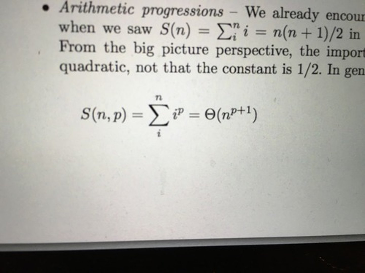
Arithmetic progressions

For p < -1, this sum always converges to a constant.