Producer theory

Firm definition

An organisation that transforms inputs into outputs (production definition) to meet consumer demand and generate profit

Producer theory assumptions

• The firm produces a single good

• The firm has already chosen which product to produce

• Firms minimise costs associated with every level of production (necessary condition for profit max.)

• Only two inputs are used in production: capital and labour

• Distinguish between short run (when one or more inputs are fixed, typically capital is assumed to be fixed and amount of labour can be changed) and long run (when all inputs are variable and fully adjustable)

• The more inputs a firm uses the more output it makes

• Inputs are characterised by diminishing returns e.g. if capital is fixed then each additional worker eventually produces less incremental output than the last

• Firms are NOT budget constrained

• Production function: Q = f (K,L)

Production function:

Specifies the maximum output that can be produced with a given quantity of inputs, it’s defined for a specific state of engineering and technical knowledge

Different combinations of inputs can generate the same output - because labour and land come from different markets so have different costs, so same input combinations could come at a different price - but firms choose the least costly method to produce the target output level they want

Total product

Total output (Q) produced with a given level of input

Upward sloping concave shape graph - increases steeply at first then flattens

Average product

Total output divided by number of units of input (AP_L = Q/L) for average product of labour

Marginal product

The extra output generated from one additional unit of input, holding all other inputs constant (MPL=\frac{\Delta Q}{\Delta L}) this is marginal product of labour

Diminishes with each additional input - downward sloping convex shape graph

Returns to scale

Examines how output responds when all inputs change proportionally

Constant returns to scale

Output increases by the same proportion e.g. inputs doubled outputs doubled

Seen in small-scale manufacturing, handcrafting

Increasing returns to scale

Output increases more than proportionally e.g. inputs doubled outputs triple

Driven by specialisation, automation and fixed costs spread over larger output

Decreasing returns to scale

Output increases LESS than proportionally e.g. double all inputs output rises only by 50%

Often due to coordination issues or resource constraints

Isoquant

Curve that shows all combination of inputs that produce the same level of output - including fractional input levels e.g. 3.7 hectares - describe the trade-offs between inputs

(Show all input bundles with the same output - similar to indifference curve that show all bundles with the same utility and has similar shape - convex)

Isoquants close together reflect increasing returns to scale, and more dispersed isoquants reflect decreasing returns to scale

Marginal rate of technical substitution

Equivalent to the slope of the isoquant curve - describes the rate at which labour must be substituted for land in this case, to hold the quantity produced constant

MRTS_LA = − ∆A (Land) /∆L (Labour)

OR

MRTS_LA = − MP_L/MP_A

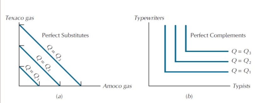
Shape of isoquants - graphs perfect substitutes/complements

If inputs are perfect substitutes isoquants would be straight lines

If inputs are perfect complements isoquants would be L shaped

Isocost line

Shows all input combinations that result in the same total cost given a fixed level of output

Higher isocost lines represent higher levels of cost

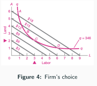
Cost minimisation - isoquant and isocost

The optimal input choice is where the ISOQUANT is tangent to the lowest possible ISOCOST line - slope of isoquant = slope of isocost

In this picture it is clear point C is the optimal choice

Firms minimise costs when the marginal product per dollar spent is EQUAILISED across inputs - equimarginal principle

Total costs formula

TC = TFC + TVC

Fixed costs

Cost that is constant regardless of output produced e.g. rent

FC = TC - TVC or FC = AFC x Q

Variable costs

Costs that change in direct proportion to output e.g. raw material costs

VC = TC - FC or VC = AVC x Q

Graph showing relationship between TC, TVC and TFC - and shape of TC and TVC explain

They are influenced by the law of diminishing marginal returns, as initially there is a decrease in cost as a variable factor of production is added to the fixed factors which increase output, until a certain point where output then falls as the fixed factors are overcrowded causing the costs to then start to increase

Average fixed cost formula

AFC = FC/Q or AFC = ATC - AVC

Average total cost formula

ATC = TC/Q or ATC = AFC + AVC

Average variable cost formula

AVC = VC/Q or AVC = ATC - AFC

Graph showing relationship between MC, ATC, AVC and AFC

Long run vs short run - cost-efficient

Long-run choices are always more cost-efficient because in the short run there is input inflexibility

Relationship between short run and long run average total cost curves

Short run cost curves are U shaped due to law of diminishing marginal returns where average costs initially decrease until a point where they start to increase. Then, in the long run all FoP are variable, and firms want to produce with the lowest cost method of production, so they will rearrange them to minimise cost - lowest point of all SRAC curves make up the LRAC curve (LRAC curve U shaped due to size of business + economics of scale)

Diseconomy of scale

As output rises average cost also rises

Economies of scale

As output increases average cost falls