Algorithms Final Exam

COP 4531 - Algorithm Design & Analysis

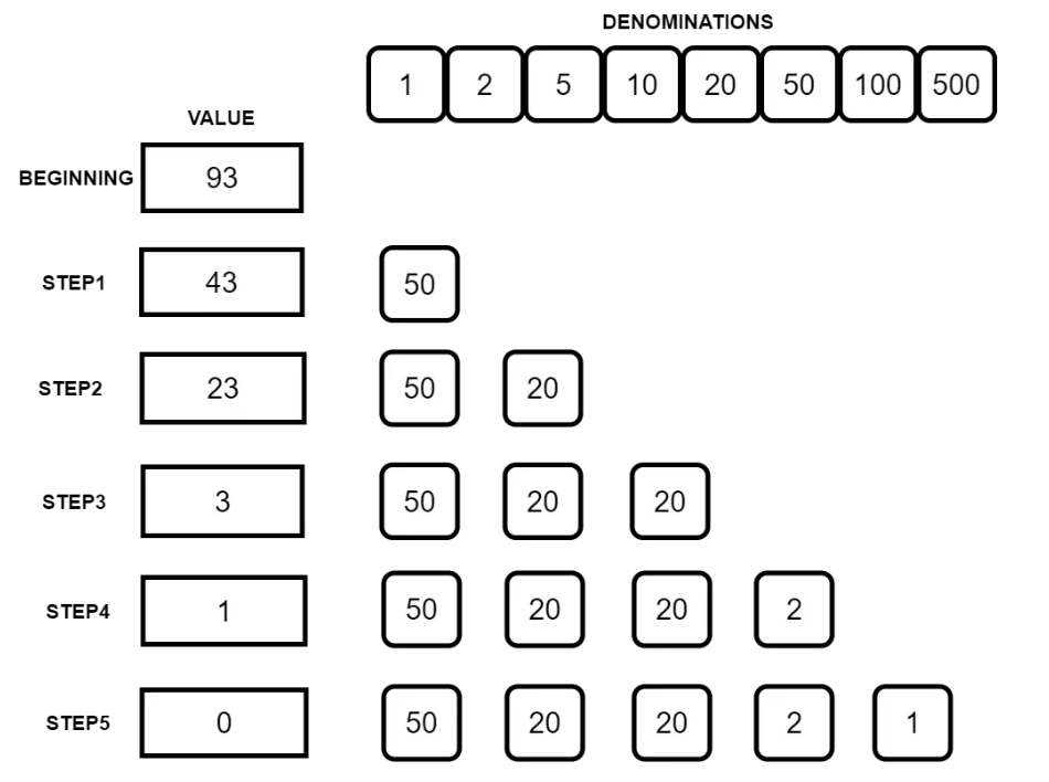
Greedy Algorithm: Coin Changing

There are scenarios in which it does not produce an optimal result!

Algorithm:

1. Sort the array of coins in decreasing order.

2. Initialize ans vector as empty.

3. Find the largest denomination that is smaller than remaining amount and while it is smaller than the remaining amount:

   • Add found denomination to ans. Subtract value of found denomination from amount.

4. If amount becomes 0, then print ans.

Time Complexity: O(n)

Greedy Algorithm: Interval Scheduling

Goal: Find maximum subset of mutually compatible jobs.

We want as many jobs as possible → earliest finish time!

Algorithm:

1. Sort the intervals by their end times in ascending order.

2. Initialize an empty schedule.

3. Iterate through the sorted intervals:

   • Add the current interval to the schedule if it does not overlap with the last selected interval.

4. Return the selected intervals as the result.

Time Complexity: O(nlogn)

Greedy Algorithm: 01 Knapsack

Goal: Get as valuable as a load as possible without exceeding weight limit.

Taking the densest items DOES NOT WORK!!! → It does not consider the possibility of excluding certain items to achieve a better overall solution. → USE DP INSTEAD

Algorithm:

1. Calculate density (value/weight) per item.

2. Sort items in descending order by their density.

3. Start with empty knapsack.

4. Traverse the sorted items and add each item to the knapsack if it fits within the remaining capacity.

5. If an item’s weight exceeds the capacity, skip it.

Time Complexity: O(nlogn)

Greedy Algorithm: Fractional Knapsack

Goal: Get as valuable as a load as possible without exceeding weight limit.

Algorithm:

1. Calculate density (value/weight) per item.

2. Sort items in descending order by their density.

3. Start with empty knapsack.

4. Iterate through the sorted items:

   • If the entire item can fit into the knapsack without exceeding capacity, take it entirely.

   • Else, take the fraction of the item that fits into the remaining capacity of the knapsack.

5. Stop when the knapsack is full.

Time Complexity: O(nlogn)

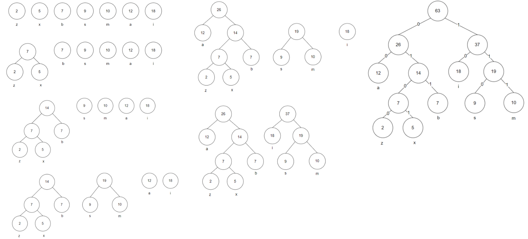
Greedy Algorithm: Huffman Encoding

Given - a:12, b:7 z:2, x:5, s:9, m:10, i:18

Ans - a: 00, b: 011, z: 0100, x: 0101, s: 110, m:111, i:10

**All Huffman encoding trees are full binary trees!!!

Algorithm:

1. Build a min heap (priority queue) where each element is a node representing a character and its frequency.

   • Nodes are ordered by smallest frequency at the top.

2. While there is more than one node in the heap:

   • Extract two minimum frequency nodes from min heap.

   • Create a new internal node with a frequency equal to the sum of the two nodes frequencies.

   • Add the new node back into the heap.

3. Repeat step 2 until the heap contains only one node. The remaining node is the root node.

4. Traverse the Huffman tree from the root to each leaf node, assigning binary codes based on the path: left branch = 0, right branch = 1

Time Complexity: O(nlogn)

Greedy Algorithm: Vertex Coloring

Goal: A coloring of the vertices using as few colors as possible.

Algorithm:

1. Start with an empty coloring.

2. Color the first vertex with the first color.

3. For each of the remaining V-1 vertices:

   • Check the colors of all its adjacent vertices (neighbors).

   • Assign the lowest numbered color that is not already used by any of its neighbors.

   • If all previously used colors appear on vertices adjacent to v, assign a new color to it.

4. Continue until all vertices are colored.

Time Complexity: O(V² + E) → worst case

Dynamic Programming: Fibonacci Numbers

Instead of using recursion to get O(2ⁿ) time, we can use the two following methods.

Memoization → O(n):

fib(n){
	if (n in memo):
		return memo[n]
	if (n<= 2):
		f = 1
	else:
		f = fib(n-1)+fib(n-2)
		memo[n] = f
		return f
}

Bottom-Up → O(n):

fib = []
fib(n){
	for (k = 1; k<=n; k++):
		if (k<= 2):
			f = 1
		else:
			f = fib[k-1]+fib[k-2]
		fib[k] = f
		return fib[n]
}

Recurrence Formula: T(n) = T(n-1) + T(n-2)

Dynamic Programming: All Pairs Shortest Path

A^k[i,j] = Cost of the shortest path from i to j using k intermediate vertices (1, 2, 3, ...k)

Recurrence Formula: A^k[i,j] = min{ A^k-1[i,j], A^k-1[i,k] + A^k-1[k,j] }

for (k = 1; k <= n; k++)
{
	for(i = 1; i<=n; i++)
	{
		for(j = 1; j<=n; j++)
		{
			A[i,j] = min(A[i,j] , A[i,k] + A[1,k])
		}
	}
}

Time Complexity: O(n³)

Dynamic Programming: 01 Knapsack

Recurrence Formula: T[i][j] = max{ T[i-1][j], T[i-1][j-w_i]+v_i }

Time Complexity: O(nw) where n is the number of items and w is the capacity.

Dynamic Programming: Longest Common Subsequence

Recurrence Formula:

• LCS[i][j] = LCS[i-1][j-1] + 1 if X[i] = Y[j]

• LCS[i][j] = max{ LCS[i][j-1], LCS[i-1][j] } if X[i} ≠ Y[j]

Time Complexity: O(mn) where m and n are lengths of strings s1 and s2.

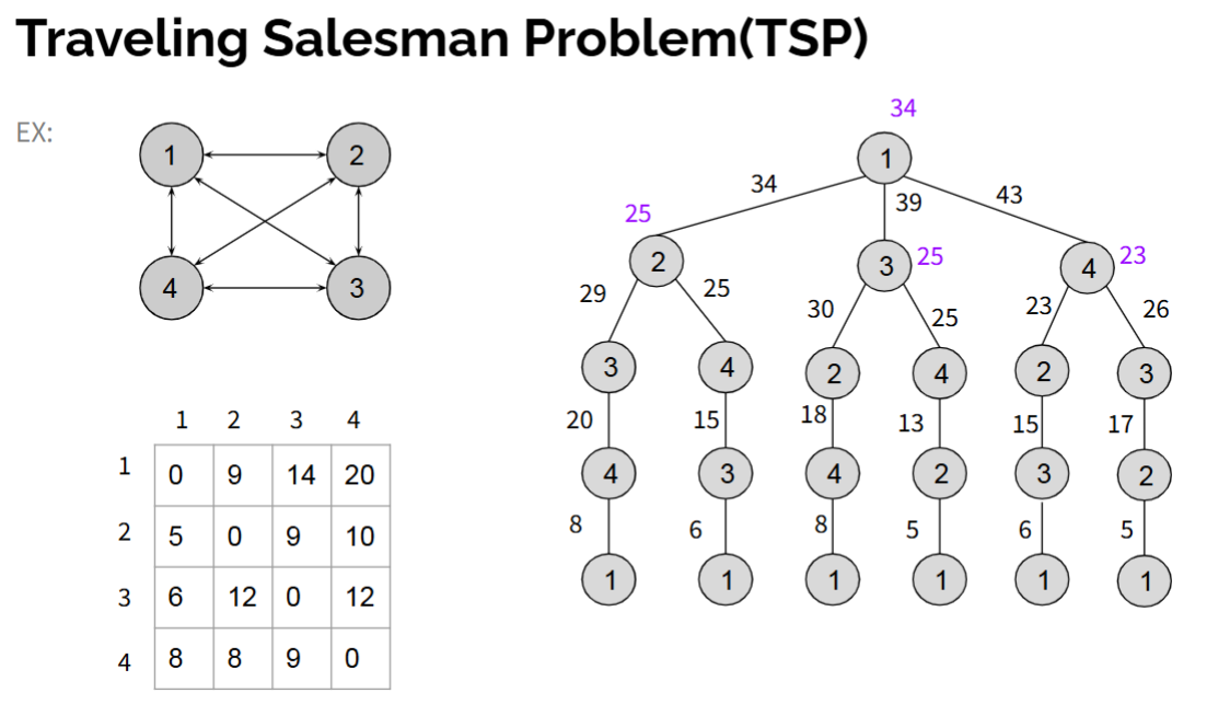
Dynamic Programming: Traveling Salesman

Input: list of cities and the distances between each pair of cities

Output: the shortest possible route that visits each city exactly once and returns to the origin city

Recurrence Formula: C(i, S) = min k ϵ S { w_ik + C(k, S-{k}) } where S is set of vertices

Time Complexity: O(2ⁿ*n²)

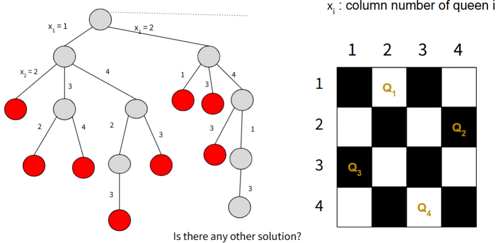
Backtracking: N Queen

Time Complexity: O(N!)

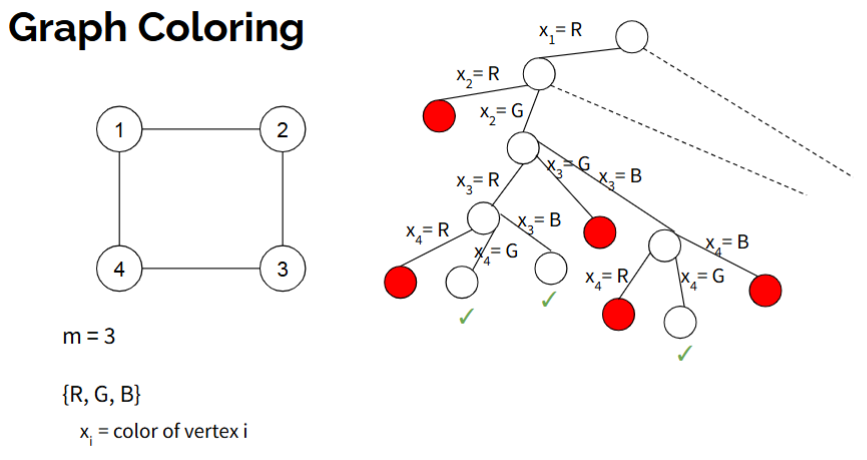
Backtracking: Graph Coloring

Time Complexity: O(m^V)

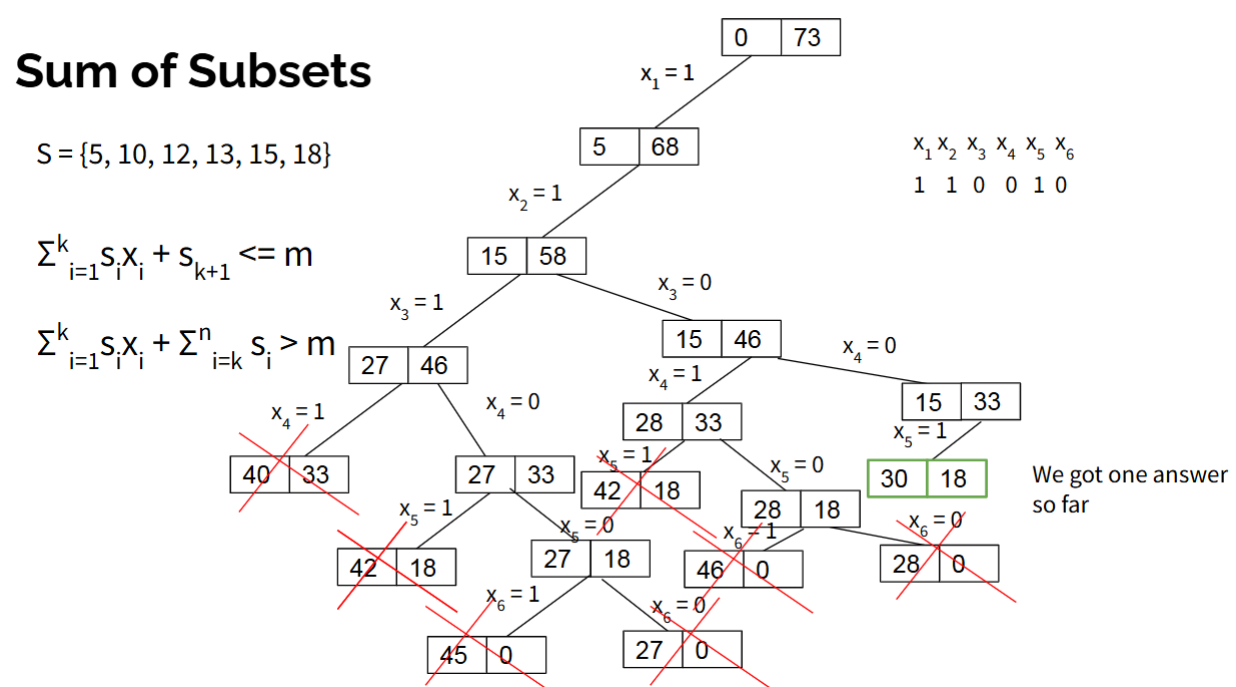
Backtracking: Sum of Subsets

Given m = 30 so if the current weight is not equal to 30, kill the node.

Time Complexity: O(2ⁿ)

Branch and Bound: 01 Knapsack

Time Complexity: O(2ⁿ)

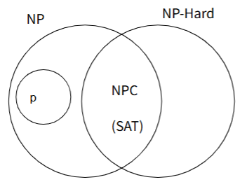
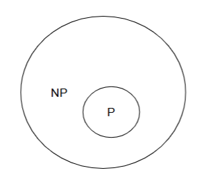
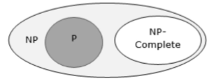
Class P

• Set of deterministic algorithm which take polynomial time

  • EX: Binary Search, Huffman Coding, Insertion Sort, Minimum Spanning Tree and etc.

• Do problems such as traveling salesperson and 0/1 Knapsack (no polynomial-time algorithm has been found), etc., belong to P? → No one knows

• To know a decision problem is not in P, it must be proven it is not possible to develop a polynomial-time algorithm to solve it

Class NP

• The set of decision problems solvable in nondeterministic polynomial time. The output of these problems is a YES or NO answer.

• Nondeterministic → a solution can be guessed out of polynomially many options in O(1) time. If any guess is a YES instance, then the nondeterministic algorithm will make that guess.

• Set of non-deterministic algorithm which take polynomial time

  • There exists polynomial time verification algorithm for them

  • EX: 0/1 Knapsack problem, Hamiltonian path problem, Travelling salesman problem and etc

NP-Complete

• A subset of NP (nondeterministic polynomial time) problems.

• If you can find a polynomial-time algorithm to solve any NP-complete problem, you can also solve all problems in NP in polynomial time. In other words, NP-complete problems are the "hardest" problems in NP in terms of their potential to be solved efficiently.

• They are both in NP and have the property that any problem in NP can be reduced to them in polynomial time.

• Ex: Determining whether a graph has a Hamiltonian cycle, Determining whether a Boolean formula is satisfiable(SAT problem)

NP-Hard

• NP-hard problems are a broader category of problems that may or may not be in NP.

• They are at least as hard as the hardest problems in NP.

• Unlike NP-complete problems, NP-hard problems do not necessarily belong to NP. It's possible that an NP-hard problem is not in NP, which means that there may not be an efficient algorithm to verify a proposed solution in polynomial time.

• However, if you can solve an NP-complete problem in polynomial time, you can use that solution to solve an NP-hard problem in polynomial time as well.

• A problem is NP-hard if all problems in NP are polynomial time reducible to it. (EX: Traveling Salesman)