Microeconomics Midterm II

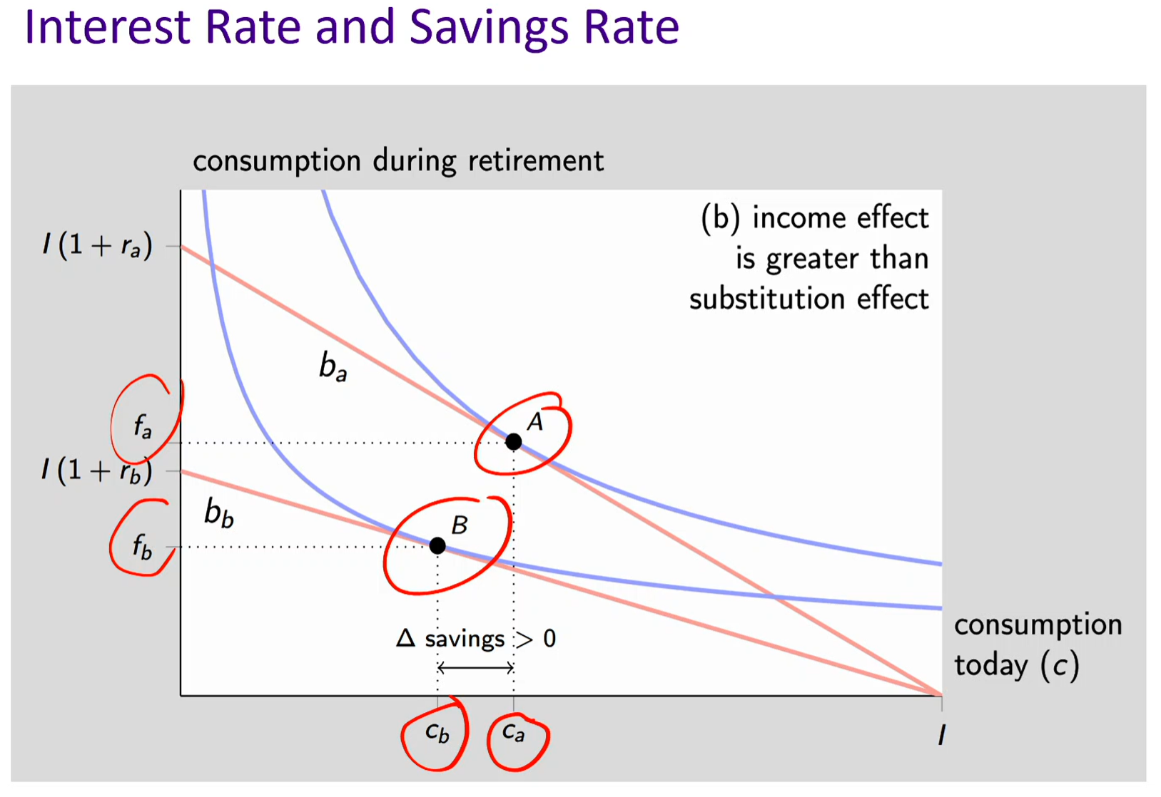
Interest rate and savings rate (Substitution effect dominates income effect)

Same concept as the first midterm

• You’re giving up Y for an additional unit of X

• You’re giving up R (return on investment) for more consumption today

In this graph, the substitution effect is greater than the income effect AND the interest rate has decreased. The budget line rotates inward/downward.

• Since interest rate has decreased, its value became cheaper. Future consumption has become cheaper to give up, so your opportunity cost has gone down (you’re giving up less Y for X)

  • Lower returns make future consumption more expensive

  • Current consumption becomes more attractive

  • Leads to INCREASED current consumption (DECREASED savings)

  • Consumer takes advantage of lower opportunity cost to consume more today

• Ex: You give up only $1.05 of future consumption, instead of $1.1. So you’re sacrificing less future consumption for every dollar you consume today. Therefore, it’s “cheaper” to consume now (because you give up less of tomorrow).

• Then, you substitute into what’s cheaper, consumption today. So you consume more today and less in the future. 

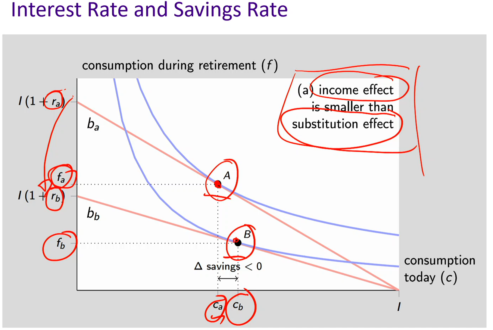
Interest rate and savings rate (Income effect dominates substitution effect)

In this graph, the substitution effect is smaller than the income effect AND the interest rate has decreased. The budget line rotates inward/downward.

• Since interest rate has decreased, its value became cheaper. Future consumption has become cheaper to give up, so your opportunity cost has gone down (you’re giving up less Y for X)

  • Lower returns reduce future consumption potential

  • If future consumption is very important, consumer compensates by saving MORE today

  • Leads to DECREASED current consumption (INCREASED savings)

• When the interest rate drops, you’re worse-off because your real income decreases, so your purchasing power decreases. Therefore, the individual is choosing to save more today (consume less today) in order to consume more during retirement.

Life-cycle optimization (intertemporal substitution motive)

A framework for understanding savings as a choice between consumption today and consumption in the future, optimizing across different periods of life

• Retirement planning: trading off current consumption for future retirement consumption

• If you save today, future consumption = I(1 + r), where I is income and r is the interest rate

Precautionary motive

The motivation to save money to build up a reserve against unforeseen contingencies or emergencies 

• Saving money for unexpected medical expenses, job loss, et

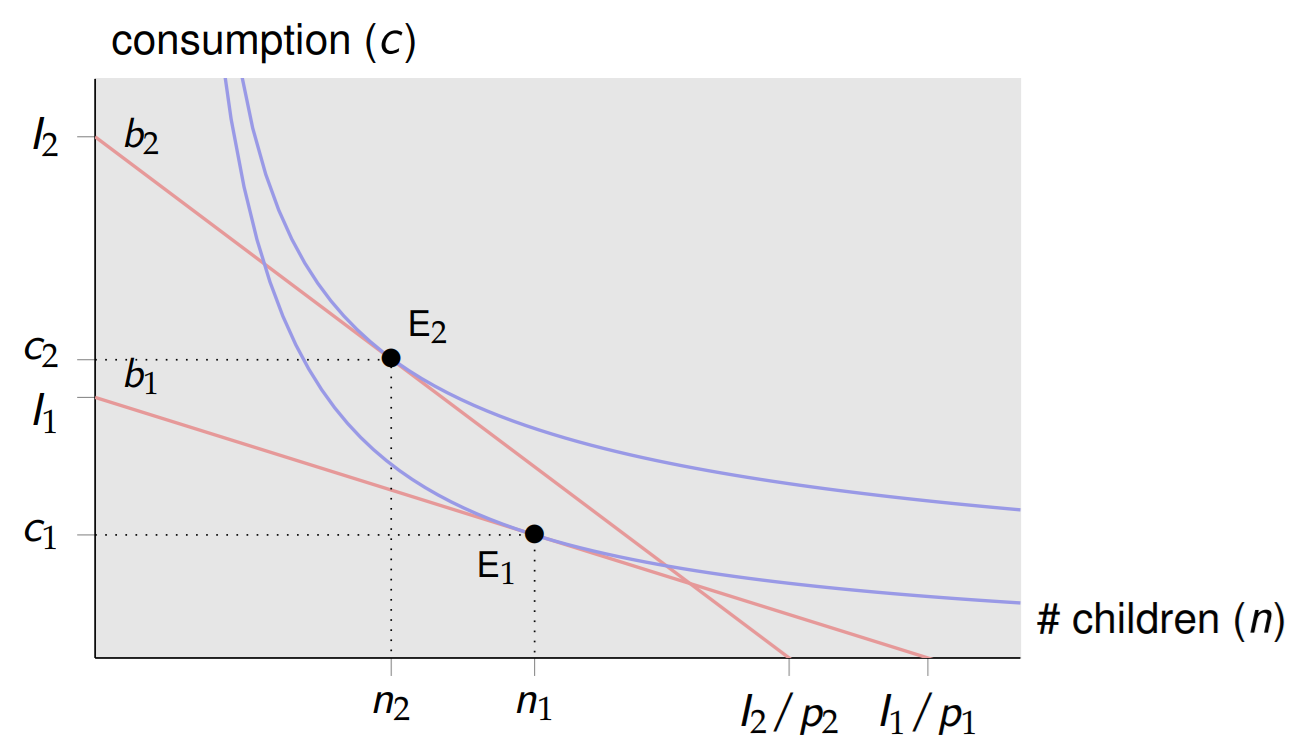
Fertility decisions

There’s a trade-off between children and consumption in dollars

• Population: ~4 billion (1968) → ~8 billion (2020)

• Fertility rate: >5 children/woman → 2.5 children/woman

• Per-capita GDP: $5,000 → $11,000 (more than doubled)

Components of Child "Price"

Direct Costs:

• Food, housing, clothing

• Schooling and education

• Healthcare

Opportunity Costs:

• Mother's personal cost of childbirth

• Foregone labor income from time spent with children

• THIS IS THE BIGGER FACTOR, especially as women's education and job opportunities improved

Children are like normal goods: higher income → more children

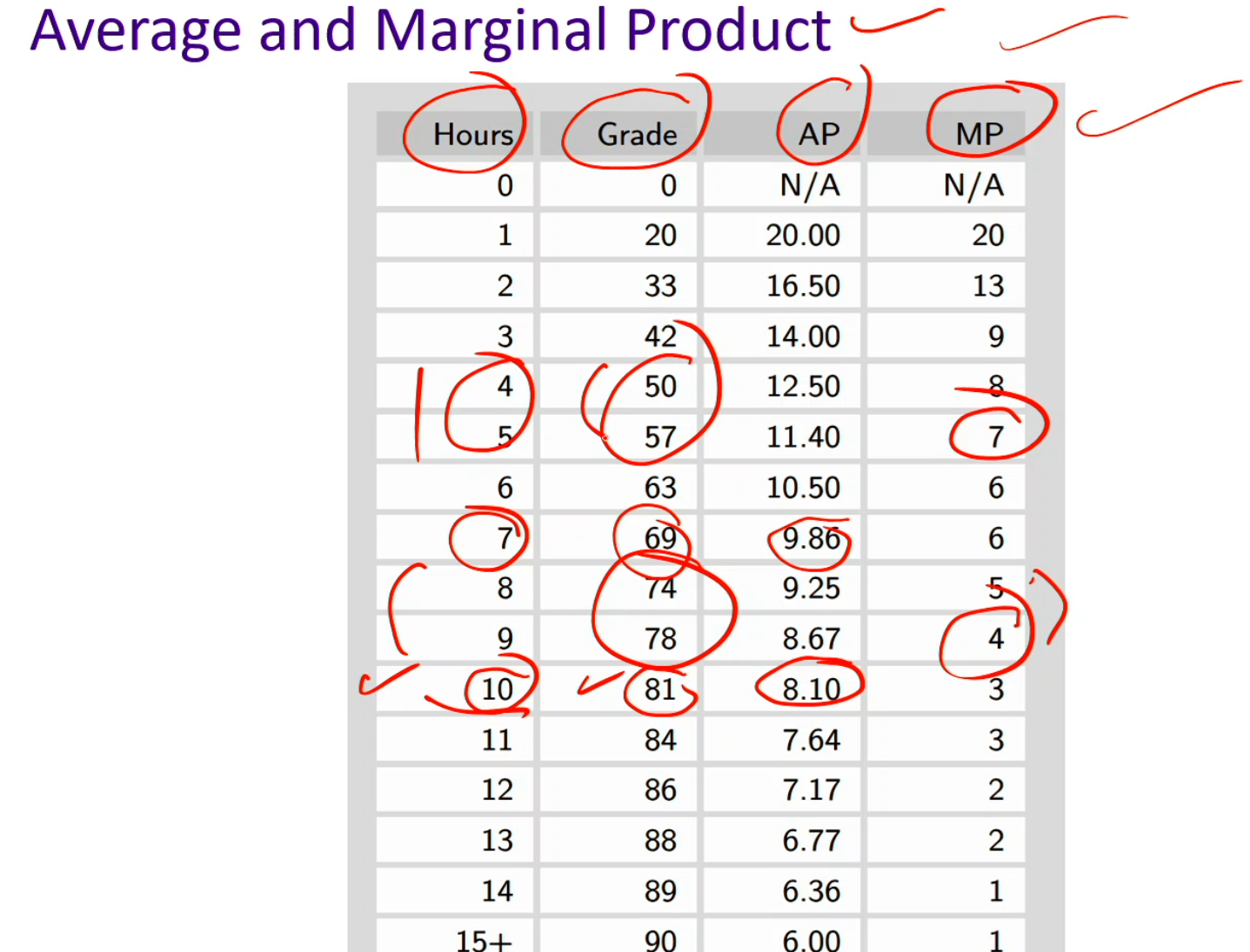
Average and marginal product

Average product: measures the average output per unit of input, how productive each unit of input is on average.

• AP = Y / X

• AP = grade / hours 

Marginal product: measures the extra output gained from one more unit of input.

• MP = Y2 - Y1 

• Ex: if you study one more hour at 4 hours to 5 hours, your MP is 7 because your grade increased from 50 to 57

• Since it’s concave, each additional X contributes less improvement then the last one

Marginal of diminishing returns:

• AP and MP decreases because as X increases, their output becomes smaller and smaller

• Ex: if you hire too many cooks, each of their contributions to the kitchen (output) decreases

• Decreasing MP implies decreasing AP (because each new unit contributes less than the average so far, it pulls the average down)

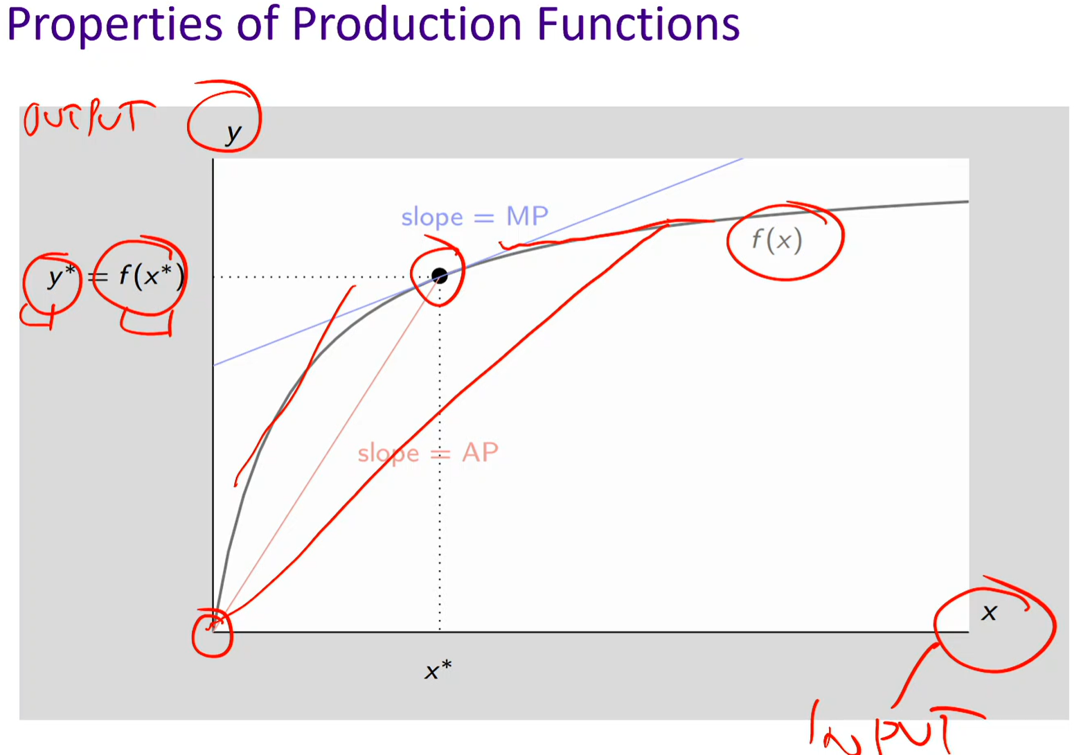
Properties of production functions

MP (Marginal product): 

• Graphically, it’s the slope of the tangent line to the production function at a given point

• MP is decreasing (each additional unit contributes less than the previous one)

  • If the tangent line at x is steep → output is growing fast → MP is high

  • If the tangent line is flat → output barely increases → MP is low

AP (Average product):

• Graphically, it’s the slope of the straight line connecting the origin (0,0) to the point

• AP is decreasing (as you add more input, the average contribution per unit declines)

  • If that line is steep → high output per unit of input (high AP)

  • If it’s flatter → low output per unit (low AP).

• When MP > AP → AP is increasing

• When MP < AP → AP is decreasing

• When MP = AP → AP is at its maximum

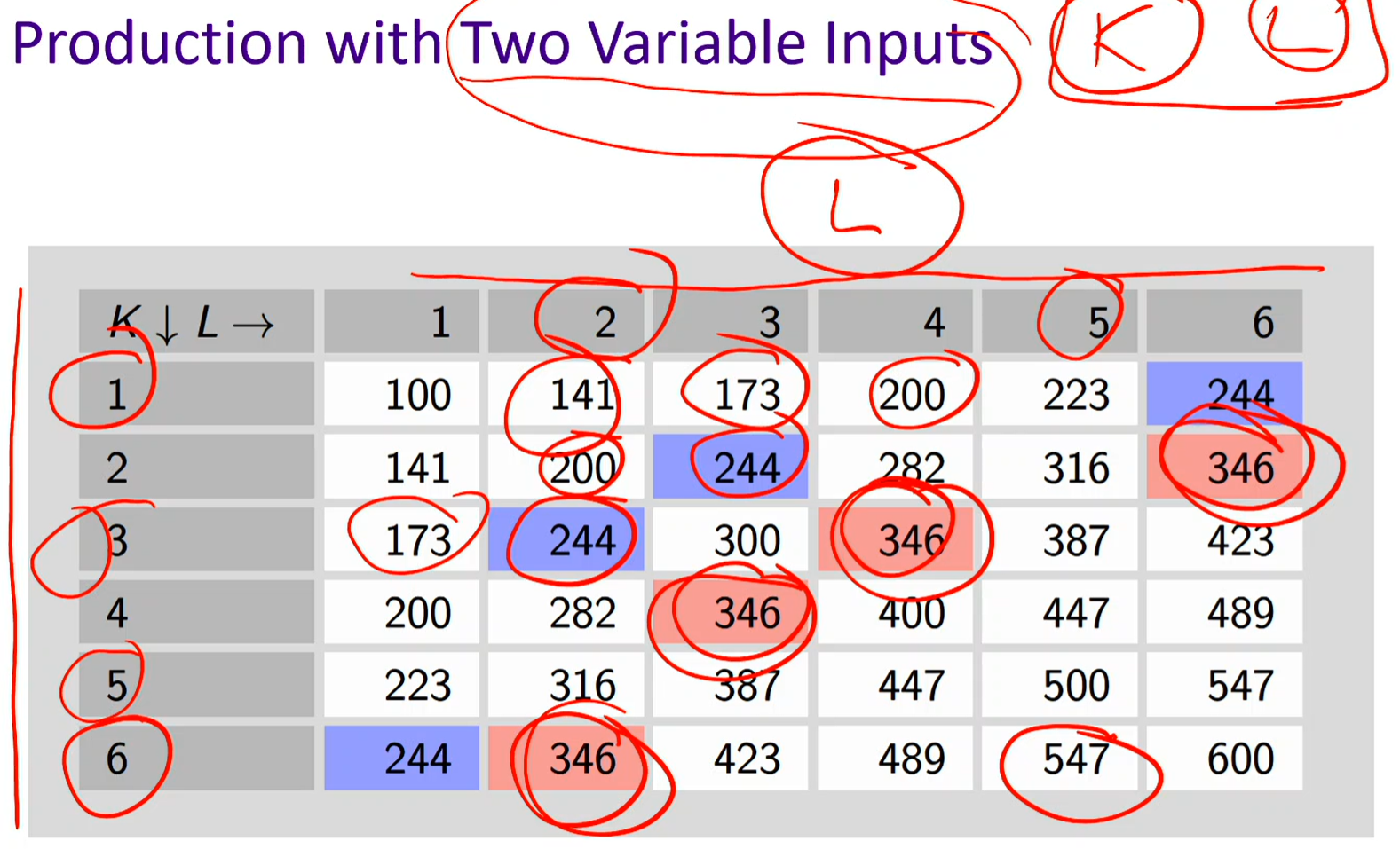
Production with two variables

In this graph:

• Different combinations of KKK and LLL can produce the same total output (like 346).

• Parallel to consumer theory: Indifference Curve: combinations of goods (X, Y) giving same utility

These are examples of: An isoquant is a curve that shows all combinations of capital and labor that yield the same output.

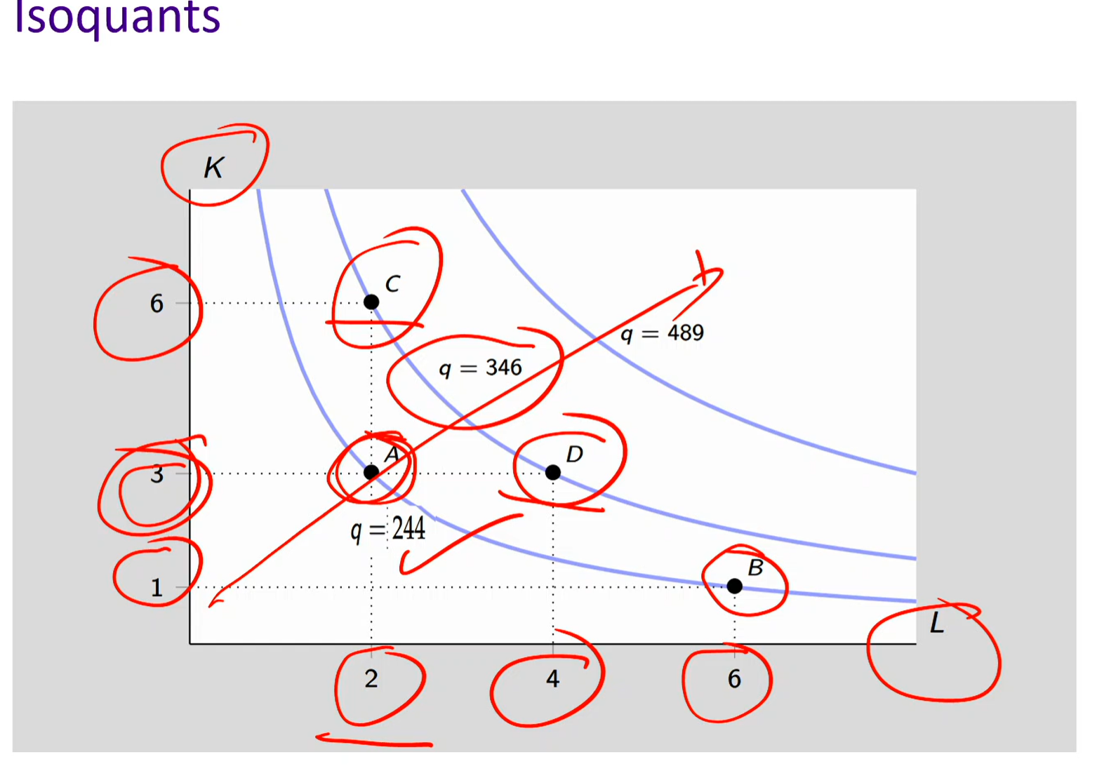
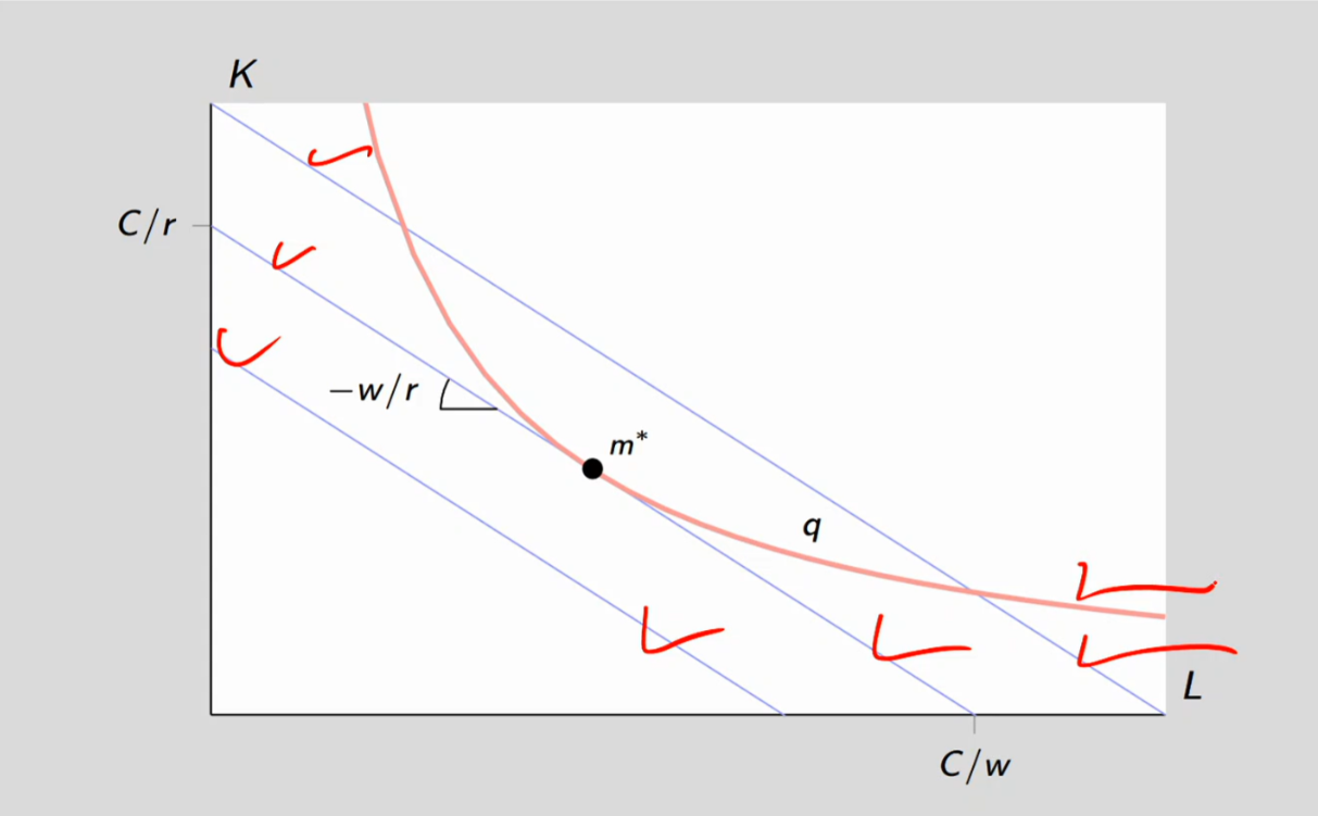
Isoquants

Isoquant: An isoquant is a curve that shows all the combinations of two inputs (usually labor LLL and capital KKK) that produce the same level of output.

Marginal Rate of Technical Substitution (MRTS): The slope of the isoquant, how much capital (K or Y) you are WILLING to give up for one more unit of labor (L or X) while keeping output constant.

• Same concept as slope of the indifference curve/MRS, BUT instead of keeping utility constant, it’s output

• A & B on same indifference curve → Equal utility (same happiness)

• Different X and Y values → Trade-off between goods

• Slope at each point (MRS) → Rate at which you’re willing to substitute Y for X

• Higher curve → More utility

• Lower curve → Less utility

Perfect Substitutes:

• Meaning: Labor and capital can replace each other completely at a constant rate

• Shape: Straight line isoquant

• Ex: Supermarket checkout (person vs. automated machine can do the same job)

Perfect Complements:

• Meaning: Inputs must be used in fixed proportions — one can’t replace the other.

• Shape: L-shaped isoquant

• Ex: Airplane flights: exactly 1 pilot + 1 plane required (more pilots without planes = useless)

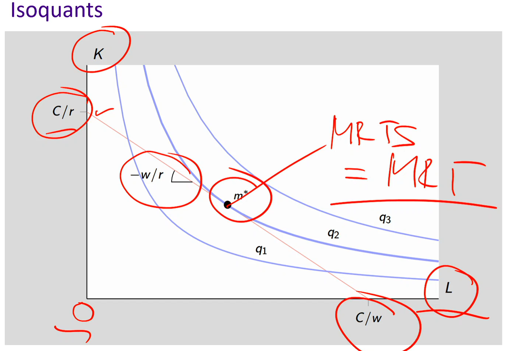
Iso-cost line

Iso-cost line: A line showing all combinations of inputs (K, L) that cost the same total amount C.

The iso-cost line comes from the firm’s total cost equation: C = wL + rK

• C = total cost (fixed amount of money the firm can spend)

• w = wage rate (cost of one unit of labor)

• L= units of labor

• r = rental rate of capital (cost of one unit of capital)

• K = units of capital

The iso-cost line is conceptually like the budget line

• Vertical intercept: C / r: the most capital the firm can afford if it hires no labor.

• Horizontal intercept: C / w: the most labor the firm can afford if it rents no capital.

Slope of the iso-cost line: w / R = MRT

• How many units of capital (K) the firm must give up to hire one more unit of labor (L) AT THE SAME COST (not output)

At m*: MRTS = MRT

• The isoquant (same output) and the iso-cost (same cost) are equal and their slopes are equal.

• At - w / r: the slope is with respect to labor over the price of capital

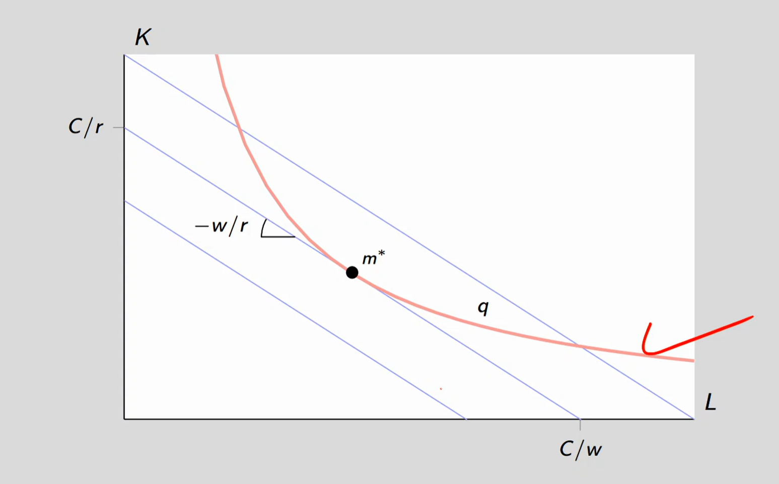
Maximize output for a given cost: You have a fixed budget (isocost line) and want to produce as much output as possible.
→ Graphically: move to the highest isoquant you can reach while staying on that isocost.

Minimize cost at a given output level: You must produce a fixed level of output and want to spend as little as possible.
→ Graphically: move to the lowest isocost that touches that isoquant.

AI, Robots, and Jobs

Computation costs have declined over time

• The Digital Revolution and its three stages:

  • Microprocessor and cheap computing

  • Internet

  • AI

• Impact on jobs and inequality

• The Core Issue: Is the new technology a substitute for labor or a complement to labor?

  If Substitutes: Technology eliminates jobs in that sector If Complements: Technology creates more jobs

  General Pattern (Historical): Technological progress eliminates jobs but doesn't increase unemployment (new jobs created as old ones destroyed)

Lower Cost of Capital

Digital Revolution largely characterized by drop in cost of capital. What impact on demand for labor

• Simple test: for the same input expenditure, does optimal input mix imply more labor or less labor?

• In present case, exactly the same, but could be higher or lower, depending on shape of isoquants

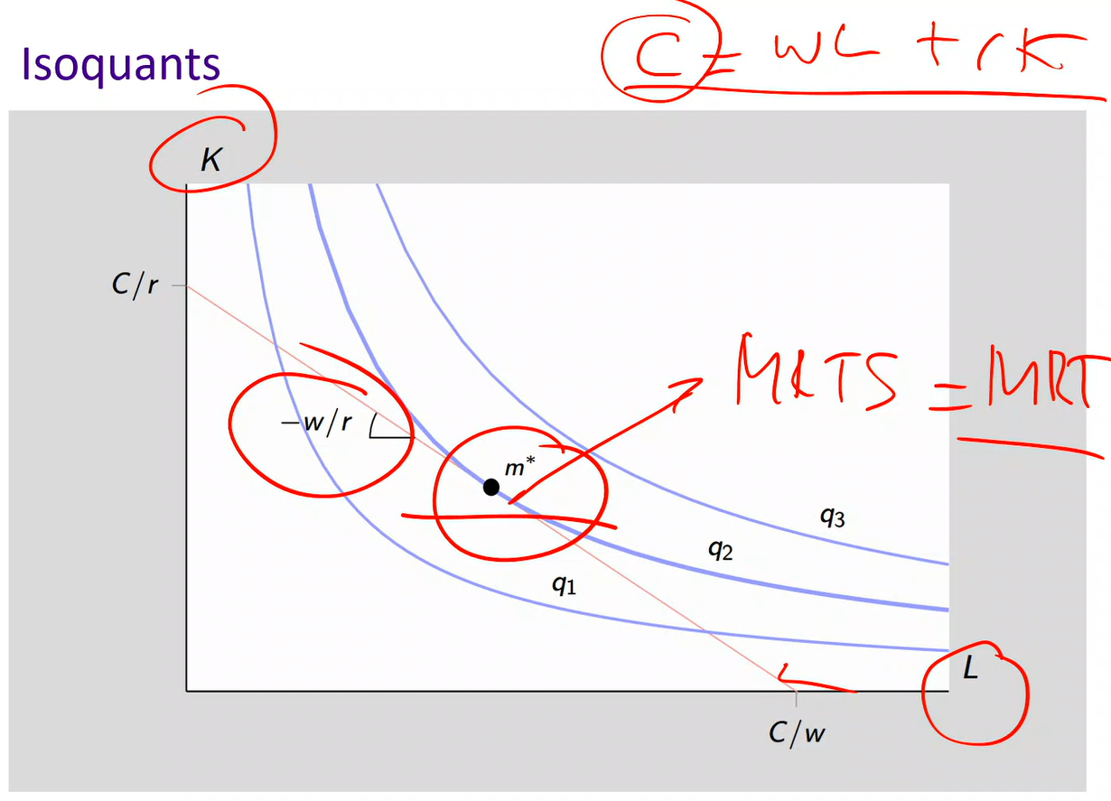
Maximize output for a given cost level vs. Minimum cost at a given output level

Maximize: 

• You fix one cost level → meaning one isocost line

• There are multiple isoquants (q₁, q₂, q₃) representing different outputs

• You ask: “With this one budget, which isoquant (output level) can I reach?”

• So you “push” the isocost line upward until it’s tangent to the highest possible isoquant

• That tangency point = maximum output given that cost

Minimize:

• You fix one isoquant → meaning one required output level

• There are multiple isocost lines (different total costs)

• You ask: “What’s the lowest-cost line that still reaches this output level?”

• You move the isocost line inward until it just touches the isoquant (tangent)

• That tangency point = minimum cost given that output

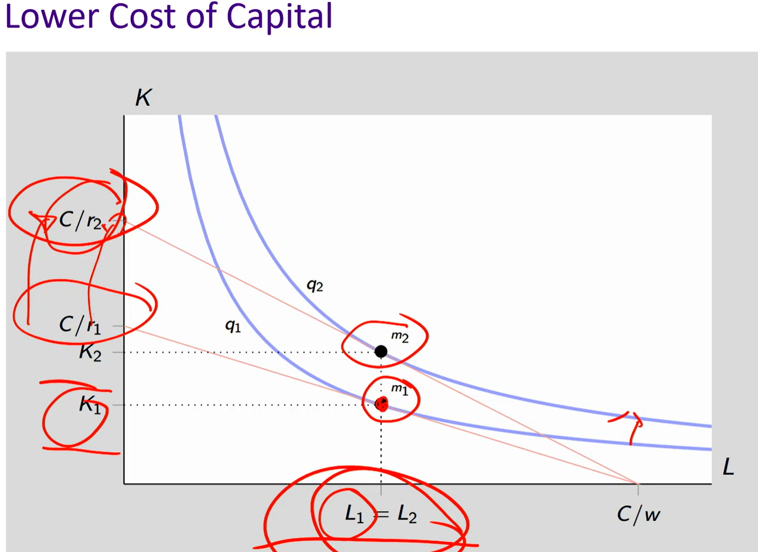
Lower cost of capital

Due to the digital revolution, technology has gotten cheaper → lower cost of capital

• r (rental rate/cost of capital) decreases so as the denominator of C / r decreases, C / r increases

• The iso-cost line pivots outward because we can buy more units as costs have gotten cheaper

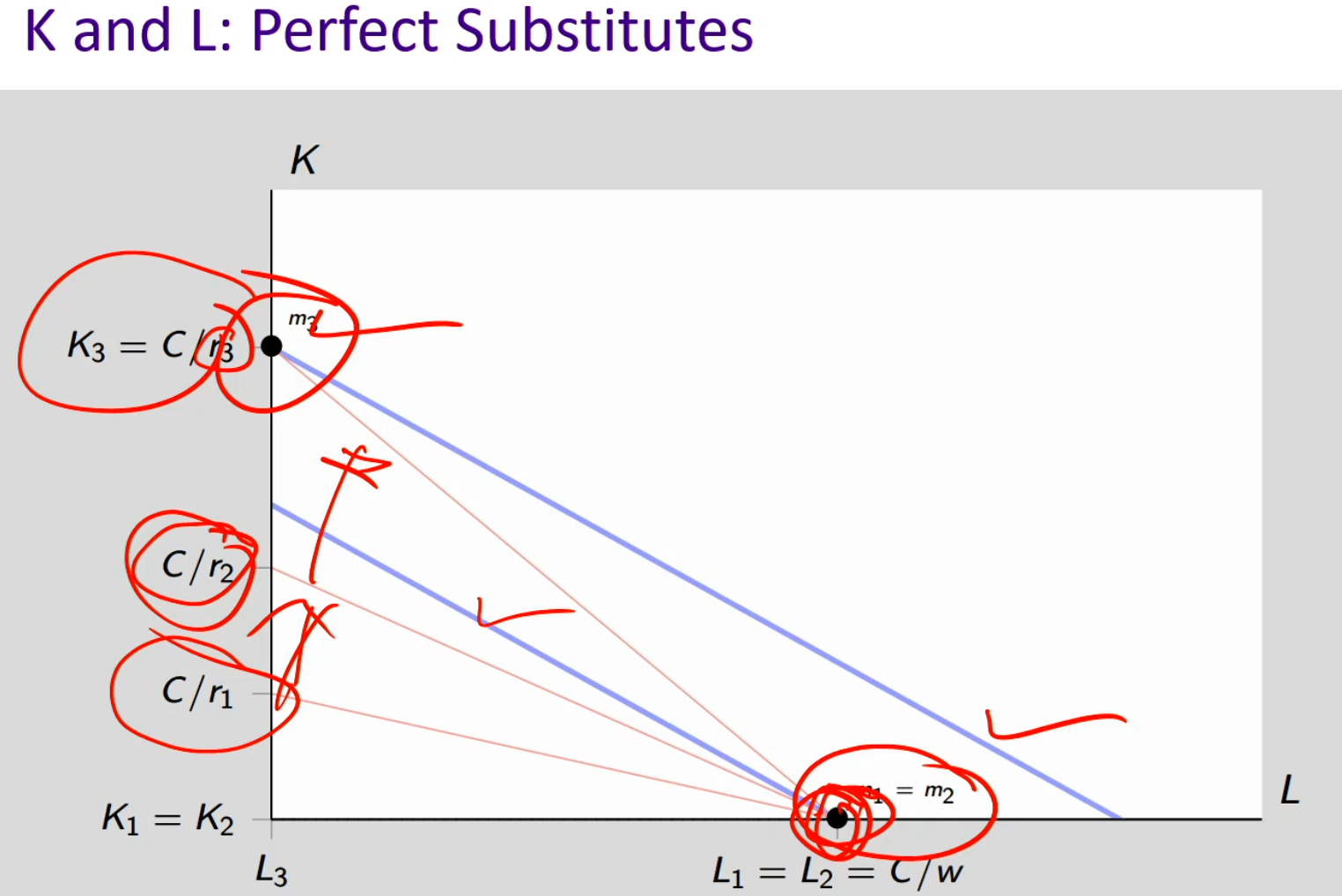
K and L: perfect substitutes

If K and L are perfect substitutes, the firm views them as equally productive per unit (like 1 unit of K = 1 unit of L)

• The isoquant (blue lines) will be linear, not curved: meaning the firm is always willing to perfectly swap one input for another at a constant rate

If labor is cheaper (w < r), the firm hires only labor → uses 100% labor, 0 capital. If capital becomes cheaper (r < w), the firm uses only capital → 0 labor, 100% capital.

• When r = r₁ (high) → capital is expensive, so the firm minimizes cost by using all labor

• As r falls to r₂, capital becomes cheaper → the iso-cost line flattens

• When r = r₃ (low) → capital is cheapest, so the firm switches to all capital (K = C/r₃)

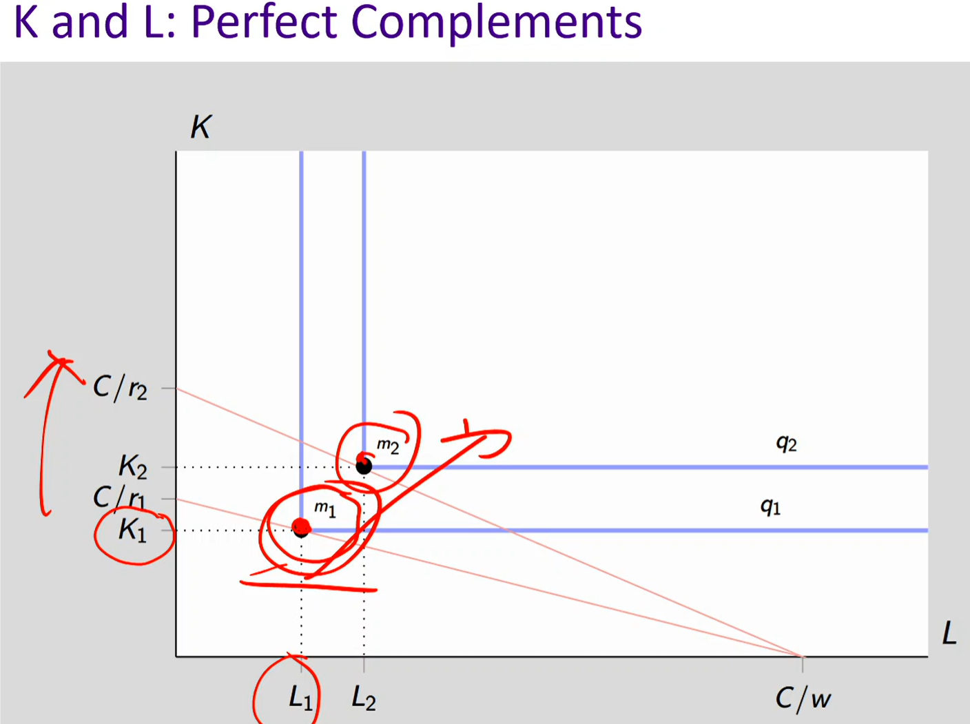
K and L: perfect complements

Perfect complements = inputs must be used together in fixed proportions

• Think of it like: 1 machine (K) + 1 worker (L) = 1 unit of output

• Adding extra of one input alone does nothing, you need both

• So the isoquants are L-shaped, because:

  • On the horizontal or vertical parts, adding more of only one input doesn’t increase output

  • Output only rises when both inputs increase together — moving to the next “corner” of the L

When cost of capital decreases, the iso-cost line pivots outwards

Example:

• The corner of the “L” is where you have the exact ratio needed (say 1 grill and 1 cook).

• Moving horizontally (more labor, same capital) → output stays constant because you’re still limited by capital.

• Moving vertically (more capital, same labor) → output also stays constant because you’re limited by labor.

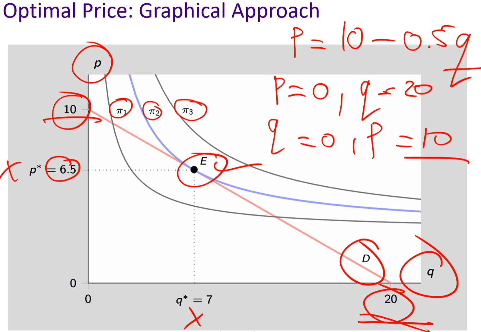
Inverse demand curve

MRT: Slope of the inverse demand curve: p = 10 -.5q

MRS: Slope of the iso-profit curve

Given demand equation (in quantity form): q = 20 - 2q

• price is the x-axis whereas quantity demanded is the y-axis

Add 2p to both sides: 2p + q = 20

Subtract q from both sides: 2p = 20 - q

Inverse demand equation: Divide both sides by 2: p = 10 - .5q

• quantity demanded is the x-axis while price is the y-axis

• price depends on quantity demanded

  • ex: at a given quantity, what price are consumers willing to pay

The seller wants the highest possible profit curve that still touches the demand curve: meaning, the optimal point E is where:

• The iso-profit curve is tangent to the demand curve: slope of iso-profit curve = slope of demand curve (MRS = MRT)

• You can’t get to a higher profit curve without going off the demand constraint

MRT = MRS implies:

∆p/∆q = (p − c)/q

The seller’s MRS

Profit function: π = (p − c) q − F

• π is profit

• p is price (price per unit the firm charges)

• c is unit cost (costs the firm incurred to produce one more good)

• q is quantity sold 

• F is fixed cost (total cost that doesn’t depend on output)

• If you increase quantity by 1 (sell one more):

  • Additional revenue ≈ p (you sell one more at price p)

  • Additional cost ≈ c

  • Net extra profit = p - c

  • Increasing quantity (selling one more) makes profit go up, because you earn p - c more on that extra unit

• If you decrease price by 1 (lower price by $1 on every unit):

  • Your revenue from each of the q units falls by $1

  • Total profit change = -q (you lose $1 × q)

  • Decreasing price by $1 makes profit go down, because you earn $1 less on each of the q units you sell, so total profit change is −q

The seller’s MRT

The seller cannot set any price and output level it wants; it must abide by the demand curve (what consumers are willing to buy at a given price)

• Ex: if you want to sell more (increase q), you must lower price (p) to get people to buy those extra units

MRT: how much price (p) would I must give up for an additional unit of quantity sold (q)

• As I increase q by one unit, I need to lower p so that consumers are willing to buy that extra unit (when the price is low, more people buy → high quantity demanded)

• MRT = the absolute value of the slope of the inverse demand curve

• In other words, MRT equals ∆p/∆q

Marginal revenue

Marginal revenue (MR): the additional revenue I get from increasing output by one unit (extra revenue from selling one more unit, after accounting for the loss from lowering price on all other units)

• When sold one more unit, you must lower the price

• In order to increase output by one unit, I need to decrease price (so as to induce consumers to buy one extra unit)

• When I set a lower price, all units I sell will be sold at a lower price

• Ex: You sell 1 cup at $10 → revenue = $10. You want to sell 2 cups → people will only buy 2 cups if price drops to $9 per cup. Total revenue from 2 cups = 2 × $9 = $18. Extra revenue from selling the 2nd cup (MR) = 18 − 10 = $8. Notice: the price of that 2nd cup is $9, but MR = $8 < $9

• Therefore, MR is lower than the p at which I sell that marginal unit

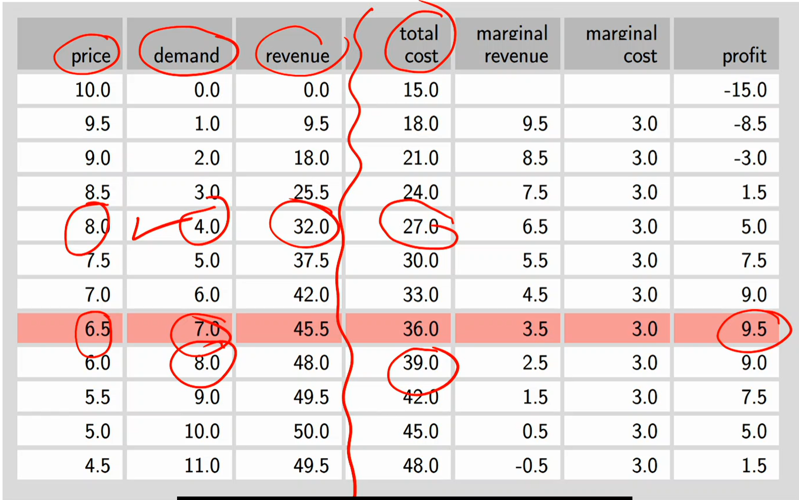
Ice-cream pricing

Marginal Revenue (MR) = how much extra revenue you get from selling one more unit

Marginal Cost (MC) = how much extra cost you incur from producing one more unit

The profit-maximizing quantity happens where: MR = MC

Revenue: price x demand

Total cost: revenue - profit

Profit: revenue - total cost

Price elasticity of demand

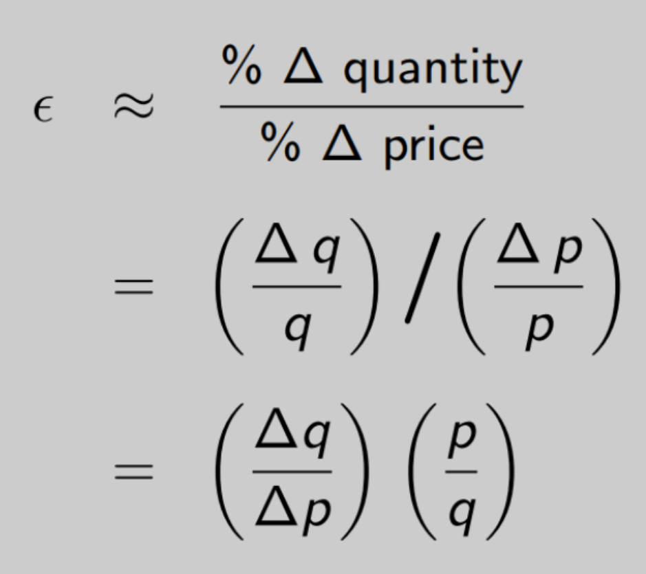
Price elasticity of demand/Epsilon: measures how much quantity demanded responds to a change in price.

% △ in quantity / % △ in price = (△ in quantity / quantity) / (△ in price / price) = (△ in quantity / △ in price) (price / quantity)

E = △q / △p (p / q)

Example:

p (price) shifts from p = 6.5 to p = 6

• Drops in price → negative .5

q (quantity demand) shifts from q = 7 to q = 8

E = 1 / - .5 (6.5 / 7) = -1.857

• When multiplying (p/q) it’s p1 and q1

Interpretation: At p = 6.5, a 1% increase (standard saying, 1% use for both increase and decrease in price) in price leads to approximately 1.857% decrease in quantity demanded

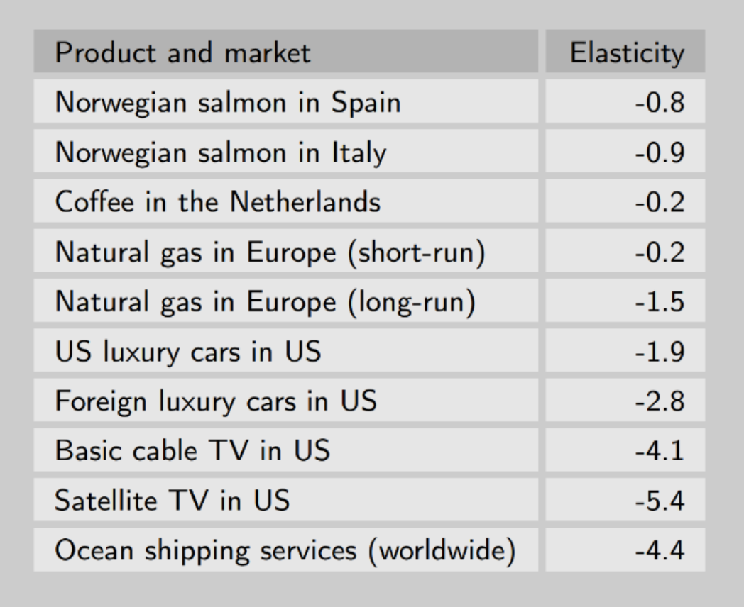
Examples of price elasticity of demand

A negative elasticity:

• obeys the law of demand: there’s a negative or inverse relationship between price and quantity demanded

  • If we raise price, quantity demanded decreases (vice versa) because the price of elasticity of demand is negative

  • If there’s NOT a negative sign, computation is wrong

Example:

• If we take per say -4.1 and take the absolute value |-4.1|, the bigger the absolute value, the bigger the elasticity. This means the more sensitive the consumers are to change in price as there’s a much bigger reaction.

More elasticities

Price elasticity of demand: sensitivity of quantity demanded with respect to a change in price/measures how much quantity demanded responds to a change in price

• If |E|> 1 = demand is elastic

• If |E| < 1 = demand is inelastic 

Income elasticity (of demand): sensitivity of quantity demanded with respect to a change in consumer income

• x = △q / △y (y / q)

• y = consumer income

• q = quantity demanded of a good

• If Ey < 0: good is inferior

  • y increases while qd decreases (vice versa)

  • (buy less when income increases)

  • Ex: instant ramen, canned foods

• If Ey > 0: good is normal

  • y increases while qd increases (vice versa)

  • (buy more when income increases)

  • Ex: brand name goods

• If Ey > 1: good is luxury

  • qd increases more proportionally as y rises 

  • Type of normal good

  • Ex: designer bags

Cross-price elasticity (of demand): sensitivity of quantity demanded of good i with respect to a change in price of good j

• x = △ qi / pj (pj / qi)

• If Eji < 0, i and j are complements

  • If peanut butter (good j)’s price increased, then its complement of jelly (good i)’s quantity demanded decreases: Pj increased while Qi decreased

  • If two goods are complements, when one gets more expensive, people buy less of both, because they are typically used together.

• If Eij > 0: i and j are substitutes

  • If energy drink (good j)’s price increased, then its substitute of coffee (good I)’s quantity demanded increases: Pj increased while Qi increased

  • When the price of one product goes up, the quantity demanded of the other product increases because people switch to it.

• If Eij = 0: i and j are independent 

  • If they’re equal to 0, they’re in the middle. The two goods have no relationships whatsoever. The cross-price elasticity = 0.

Price-margin rule

|△p / △q| = MRT

p - c / q = MRS

The price-margin rule: If the firm prices optimally, then the price-cost margin should equal the inverse of the elasticity (in absolute value)

Inverting the △ term and multiplying both sides by q / p, we get

(q / p) (1 / △q/△p) = (q / p) (p - c / q)

*Given the definition of elasticity, this is the same as - 1 / E = p - c / p*

• Left-hand side: −1 / E → inverse of elasticity (absolute value)

  • How sensitive consumers are

  • More elastic = consumers are more sensitive to price changes

• Right-hand side: (p−c) / p → price-cost margin

  • How much price exceeds cost

  • Higher price-margin = higher profit (vice versa)

Margin rule:

m = p - c / p

m = - 1 / E

MRT = MRS

- 1 / E = p - c / p could be also expressed as p = (E / 1 + E) c when solving for p

• If elasticity is high (sensitive demand) → m should be low (low markup)

  • Consumers are very price-sensitive. If you try to set a high margin, demand will drop a lot → you lose revenue.

• If elasticity is low (insensitive demand) → m should be high (high markup)

  • Consumers are not very sensitive to price. You can charge a high markup without losing many sales.

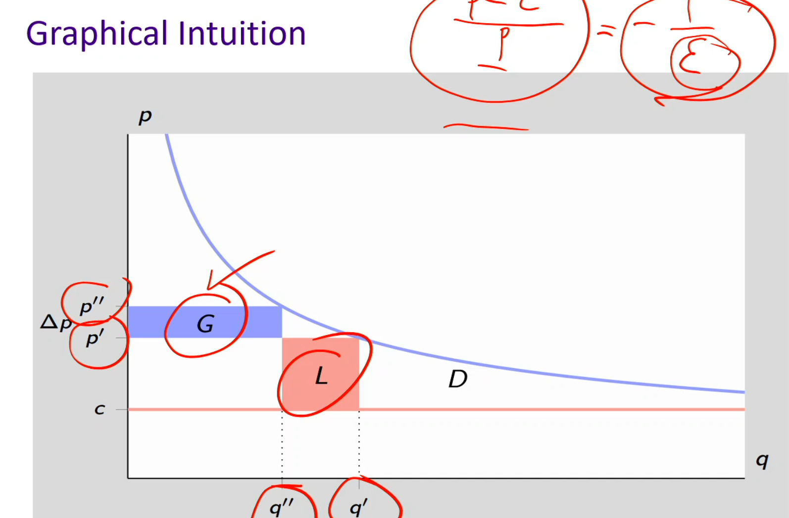
Graphical intuition

When p’ increases to p”: price increases, quantity demanded decreases

• I gain G (The extra money you make on the units you still sell after raising the price) : G is q times △ p the blue box)

• There’s also a loss of L (The money you lose because some customers stop buying due to the price increase): (p - c) (-△ q)

  • negative sign because there’s a loss of Qd at the x-axis

• G > L when q” times △ p > (p’ - c) (-△ q)

  • G > L: Raising the price increases profit only if the gain from higher price is bigger than the loss from fewer sales.

  • Rearrange this to - q △ p / p △ q > p - c / p

  • Rule: only can be rearranged if m < 1/(-E)

    • When a price increase will actually raise profit

Margin and markup

Margin: the portion of the selling price that is profit

• m = p - c / p → corresponding elasticity rules → m = 1 / -E

• Retailers evaluating their profitability, since they usually set prices based on what the market will pay and then calculate what profit they earn from it

Mark-up: the amount you add to cost to determine your selling price

• k = p - c / c → corresponding elasticity rules → k = 1 / -E -1

• How much am I adding to cost to determine the selling price

• Manufacturers and wholesalers, who  start with cost and then “mark up” to set a selling price

Example 1:

• Product: new drug, protected by patent

• Estimated elasticity: −1.5 (constant)

• Marginal cost: $10 (for a 12-dose package)

• What’s the profit-maximizing price?

• What are values of margin, markup at optimal price?

• Check elasticity rules

Profit-maximizing price: p = c / 1+ (1 / E)

10 / 1- (1 / 1.5) = 30

• When elasticity is negative, it becomes 1-1

Margin: m = p - c / p

(30 - 10) / 30 = .66 → 66%

• 66% profit

• Elasticity rule:

  • -1 / E = - 1 / - E (since given E is negative) = -1 / -1.5 = .66 → 66%

Mark-up:  k= p - c / c

(30 - 10) / 10 = 2 = 200% 

• adding 200% to cost to determine the selling price

• Elasticity rule:

  • -1 / (E + 1) = -1 / (-1.5 + 1) = -1 / -.5 = 2 = 200%

Example 2: 

• Product: cable service

• Estimated elasticity: −3.5 (constant)

• Marginal cost: $20 (per month)

• What’s the profit-maximizing price?

• What are values of margin, markup at optimal price?

• Check elasticity rules

p = c/(1+1 / E) = 20/(1-1 / 3.5) = 28

m = (28-20)/28 = 28.6%

k = (29-20)/20 = 40%

-1 / E = 1/3.5 = 28.6%

-1 (E + 1) = -1/(-3.5 + 1) = 40%

Ice-cream example:

m = 6.5 - 3/6.5 = .5385

E = 8-7/7 / 6-6.5/6.5 = 1 X 6.5 / -.5 X 7 = -6.5 / 3.5 = -1.857

1/-E = 1/1.857 = .5385

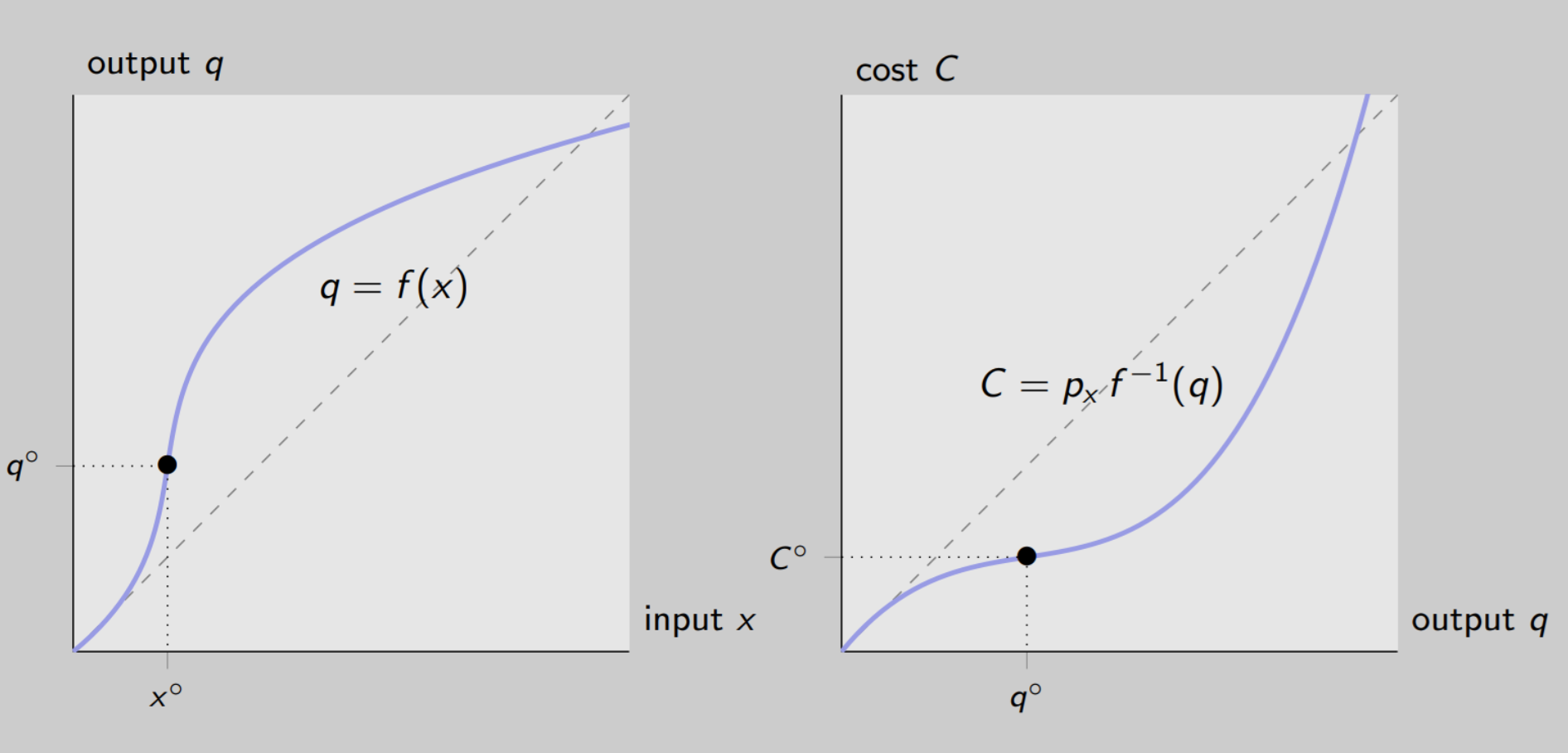
From production to cost function

Production Function Shape (Left Panel):

1) Convex portion (low input - labor) → curves upward 

• Output (goods/services produced) increases more than proportionally with input → increasing marginal product

• Why? Specialization & division of labor

  • Example: Digging holes:

    • 1 worker: slow, must do all tasks

    • 2 workers: split tasks → faster than sum of individuals

2) Concave portion (high input) → flattens out 

• Output increases less than proportionally → decreasing marginal product

• Why? Law of diminishing marginal returns

• Example: Adding too many workers: crowded, less efficient

Cost Function Shape (Right Panel):

1) Concave portion (low output) → rises slowly

• Cost rises less than proportionally as output increases → low marginal cost

• Why? Each additional unit of output can be produced cheaply because workers are highly productive

  • Example: Digging holes:

    • 1 worker: each hole is expensive

    • 2 workers: splitting tasks → cost per extra hole is lower

2) Convex portion (high output) → steepens

• Cost rises more than proportionally as output increases → high marginal cost

• Why? Producing extra units gets more expensive because adding labor/machines is less efficient → law of diminishing marginal returns

• Example: Digging holes:

  • 10 workers: crowded, slower → extra labor costs more per additional hole

Cost function

Cost function: shows the minimum total cost a firm needs to produce a given output level q, if we use the best combination of inputs. It can be characterized by:

• Fixed cost (FC): the cost that does not depend on the output level

  • Ex: rent, property taxes, salary of workers

• Variable cost (VC): that cost which is not fixed, changes with output level

  • Ex: raw materials, utilities

• Total cost (TC): the sum of fixed cost and variable cost

  • TC = FC + VC

• Average cost / Average total cost (AC/ATC) (also known as “unit cost”): total cost divided by output level

  • AC = TC / Q

  • AC = TC / Q = (FC + VC) / Q

• Average fixed cost (AFC): fixed cost divided by output level

  • AFC = FC / Q

• Average variable cost (AVC): variable cost divided by output level

  • AFC = VC / Q

• Marginal cost (MC): the cost of one additional unit. Extra cost of producing one more unit of output.

  • the change in the cost divided by the change in the output

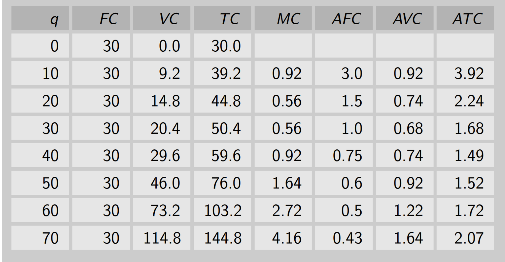
Example:

Total cost: fixed cost + variable cost

• Ex: 50.4 = 30 + 20.4

Margin cost: the change in the cost divided by the change in the output

• Ex: going from 30 → 39.2 (q is going from 0 → 10) so 39.2 - 30 = 9.2 then 9.2 / 10 = 92

Average fixed cost: FC / q

• 3 = 30 / 10

Average variable cost: VC / q

• Ex: .92 = 9.2 / 10

Average total cost: AFC + AVC

• Ex: .92 + 3 = 3.92

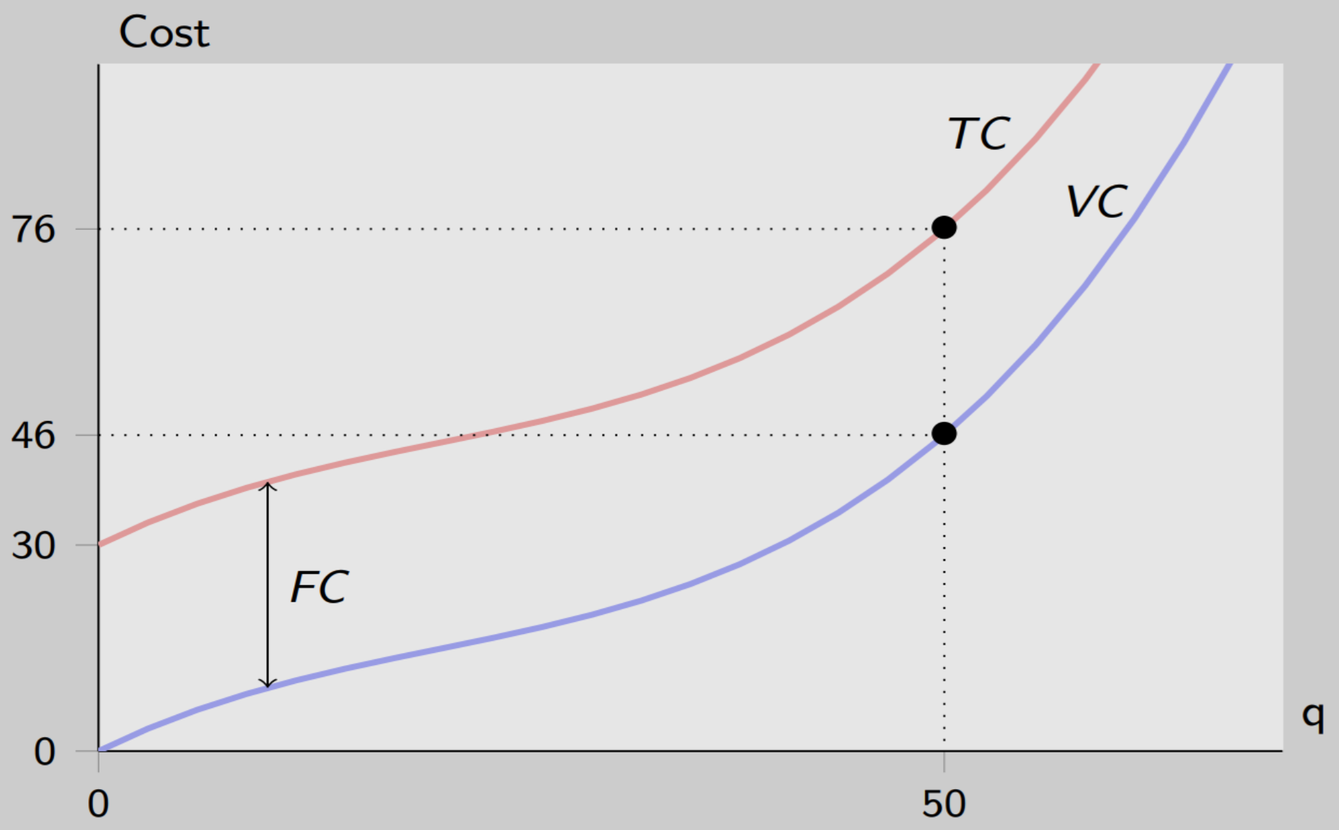
Total and variable cost graph example

There’s a vertical distance between total cost and variable cost which is fixed cost

• Fixed cost remains constant because it doesn’t change with output while total cost and variable cost changes with output

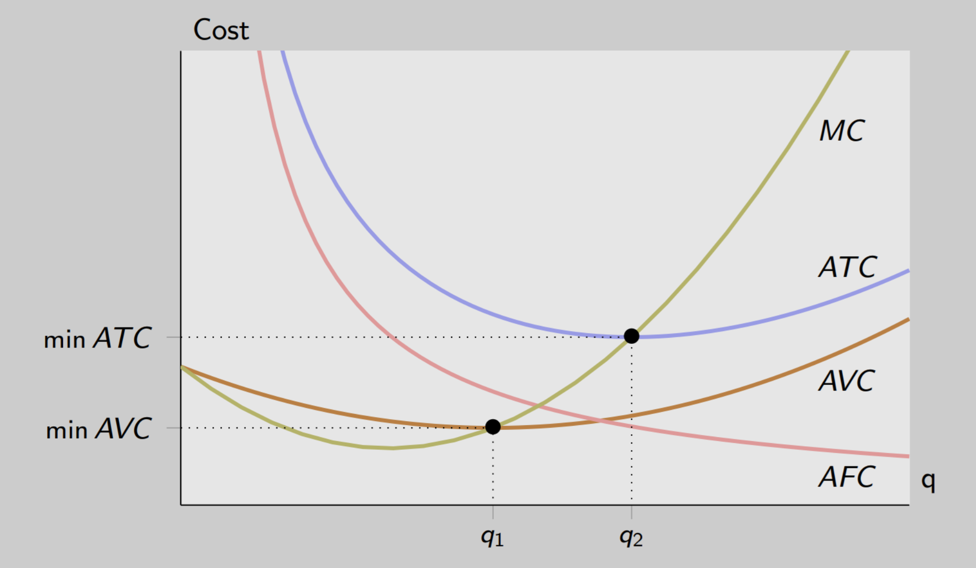
Average and marginal cost graph examples

AFC: fixed costs don’t change with output

• Always declining: As you produce more, the same FC is divided among more units → AFC falls

• At low levels of production, fixed costs are high. So when you produce more and more output from low levels of production, you spread those fixed costs over a great level of output

• Pulls down your average total cost (ATC)

AVC: U-shaped 

• At first, adding more units uses labor efficiently → AVC falls.

• After a point, diminishing marginal returns set in → each extra unit costs more → AVC rises.

• MC intersects AVC at its lowest point because:

  • If MC < AVC → producing extra unit costs less than average → AVC falls

  • If MC > AVC → producing extra unit costs more than average → AVC rises

ATC: U-shaped

• U-shaped because of economies of scales

• At low output, ATC falls because spreading FC dominates (AFC high, AVC low)

• At high output, ATC rises because diminishing returns increase MC → raises AVC → raises ATC

MC: extra cost of producing one more unit

• Intersects ATC at the minimum

• Low levels of production leads to an increased marginal cost in labor because labor is becoming inefficient due to diminishing marginal returns

• When MC is > AC, AC increases because margin drives the averages (vice versa in the beginning of the graph)

  • Ex: Your average score is like AC. Your next test score is like MC.

T-shirt factory example

In order to produce t-shirts, a manager leases one machine at the rate of $20 per week. The machine must be operated by one worker. The hourly wage paid to that worker is as follows:

• $1 during weekdays (up to 40 hours)

• $2 on Saturdays (up to 8 hours)

• $3 on Sundays (up to 8 hours)

Assuming that current output (q) is 40 t-shirts per week, we have that:

• The fixed cost is given by the machine weekly lease. We thus have FC = $20.

• The variable cost is given by 40 t-shirts times one hour per t-shirt times $1 per hour, which equals $40

• The average cost is (20 + 40)/40 = $1.50

  • Cost per unit of output

• The marginal cost is $2. In fact, producing the 41st t-shirt in a given week would imply asking the worker to work on Saturday, which would be paid at the hourly rate $2; and producing a t-shirt requires one hour of work

The factory is small relative to the market → it cannot set price. Market sets price: p = $1.80/t-shirt Factory can sell as many t-shirts as it wants at this price.

• The factory is profitable at 40 t-shirts as $1.80 > $1.50

Rule: Produce where p = MC (profit-maximizing output)

• If p > MC, produce more → gain profit on extra units

• If p < MC, produce less → avoid loss on extra units

• Since the cost of the 41st t-shirt is $2 for a Saturday wage and our revenue is $1.80, don’t produce as there’s no more profit

  • $1.80 < $2.00

• Reducing to q = 39: saves $1 (MC), loses $1.80 (price) → don't reduce

• Increasing to q = 41: costs $2 (MC), gains $1.80 (price) → don't increase

• q = 40 is optimal (p falls between MC of $1 and $2)

• Producing less → lose more revenue than you save → not optimal

• Producing more → cost exceeds revenue → not optimal

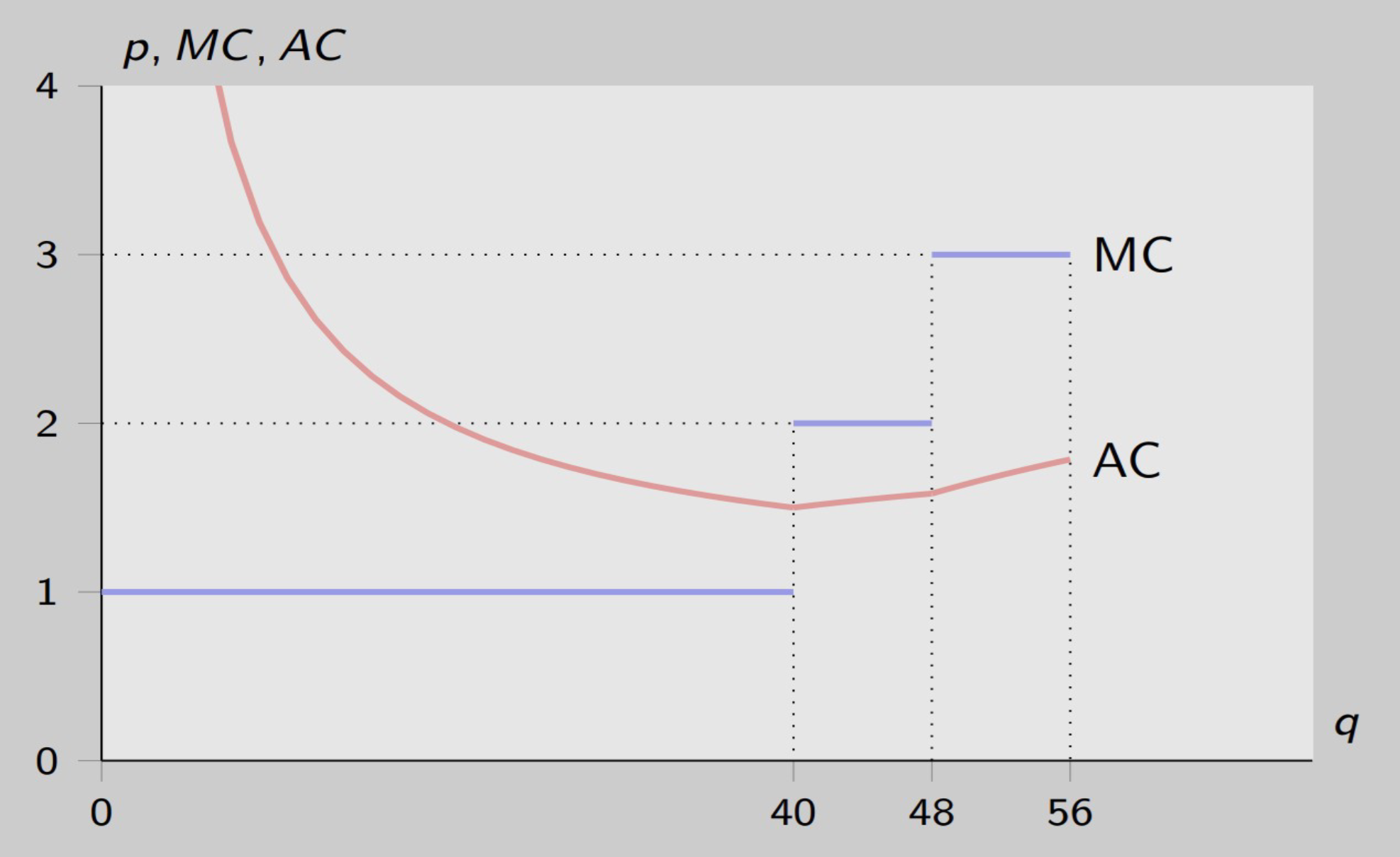
Graph:

X - outputs

Y - number of t-shirts

• $1 during weekdays (up to 40 hours)

• $2 on Saturdays (up to 8 hours)

  • 40 + 8 = 48 hours

• $3 on Sundays (up to 8 hours

  • 48 + 8= 56 hours

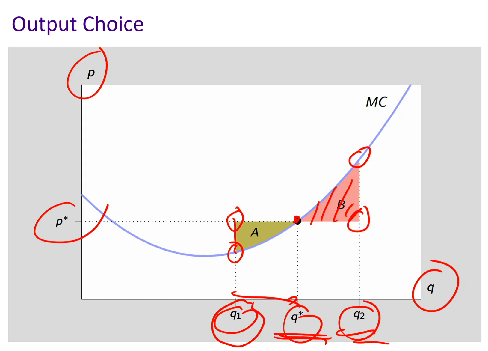
Output choice graph

Between q1 and q*, p is greater than MC

• If you simply stop at q1 and don’t progress to between q1 and q*, you’re leaving money/profit on the table

• Area A: represents forgone profit

• Producing too little → you’re missing out on profitable units

At q2, MC is greater than p

• Making a loss at between q* and q2

• Area B: represents excess losses

• Producing too much → you’re making unprofitable units

• There’s an incentive to turn backwards so you’re cutting back production from q₂ down to q* to stop losing money

Optimal Point: Where p* = MC

• Profit maximized

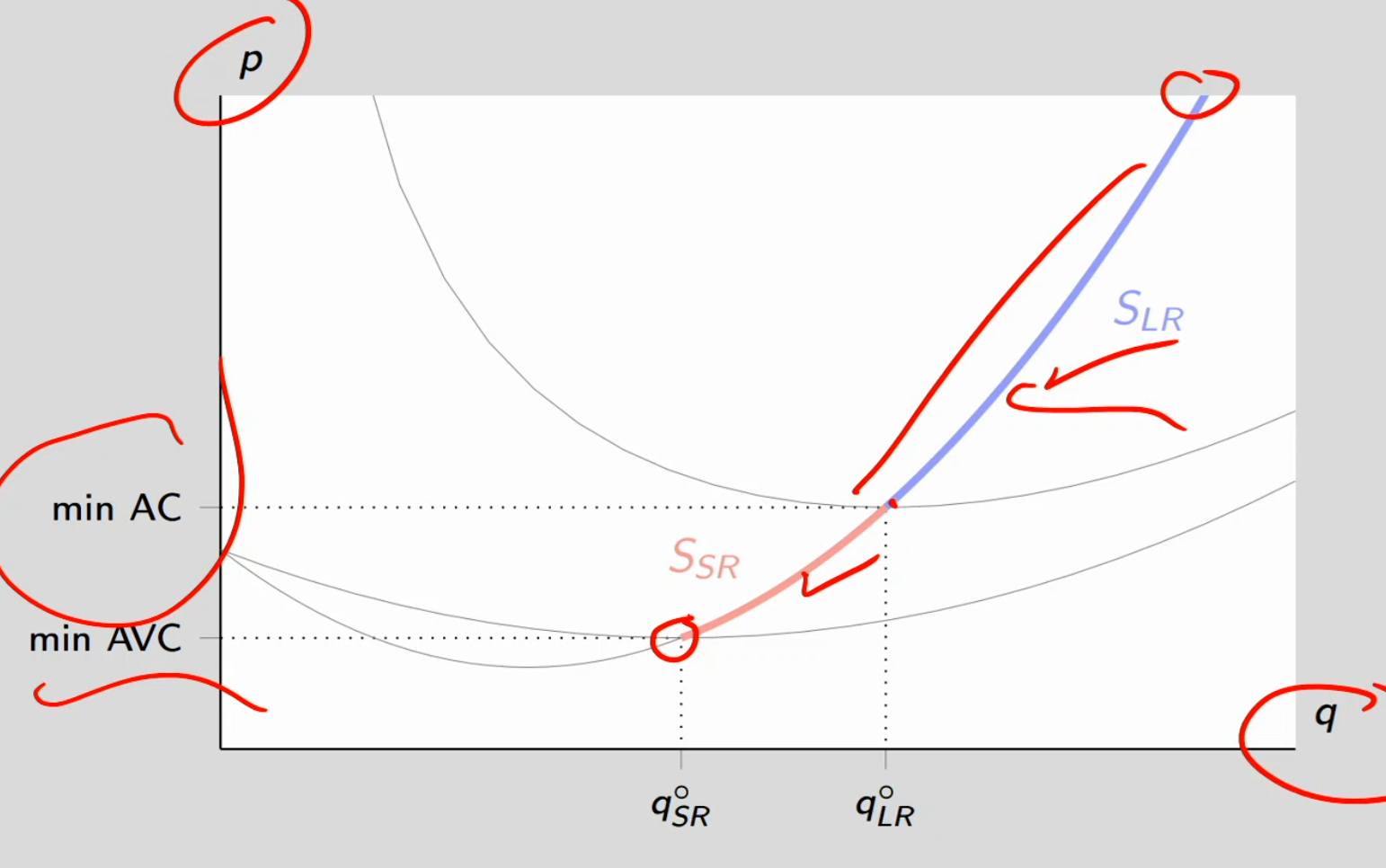
Supply by price-taking firm

Short run supply:

• Fixed costs are sunk (you’ve already paid for equipment, rent, etc.).

• The only thing that matters for staying in business right now is covering your variable costs (like labor, materials).

• If Price ≥ min(AVC) → produce where P = MC

• If Price < min(AVC) → you’re not even covering your variable costs — every extra unit you make loses money

Long run supply: 

• In the long run, nothing is fixed — firms can exit or enter the market.

• You now have to pay fixed costs again and again (rent, equipment, etc.), so you must at least cover your total costs (variable + fixed = AC)

• If Price ≥ min(AC) → produce where P = MC.

• If Price < min(AC) → exit the market permanently

Inverse supply curve 

Supply curve:

• For a given price, the supply curve corresponds to the output level that the firm is willing to supply

• Given a price, the curve tells you the quantity supplied

Inverse supply curve:

• Second, the inverse way: for a given output unit, the (inverse) supply curve corresponds to the lowest price such that the firm would want to supply that unit

• For every quantity (Q), what is the minimum price (P) the firm needs to be willing to produce it?

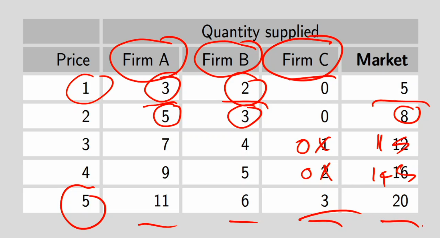
• For a given price, market supply is simply the sum of all individual firm’s supplies

  • Add up all the individual supply curves horizontally

• Note we’re adding qs for a given p, NOT adding ps for a given q

We’re asking if those different market prices, how much output will each of those firms produce

• Add up firms = market

  • Ex: at price 1, add firm A and firm B (2 + 3) = market (5)

If firms’ supply curves are given by functions of p, then we add these functions

• q = f(p)

Supply Determined by: p = MC

Therefore: Inverse supply S⁻¹(q) = MC(q)

Meaning of Inverse Supply:

• For given output level q

• Inverse supply gives LOWEST PRICE firm requires to supply that unit

• If p < MC(q): won't supply that qth unit

• If p ≥ MC(q): will supply that qth unit

Summary:

• Direct supply curve: Given p, how much will firm supply?

• Inverse supply curve: Given q, what minimum p needed to induce firm to supply it?

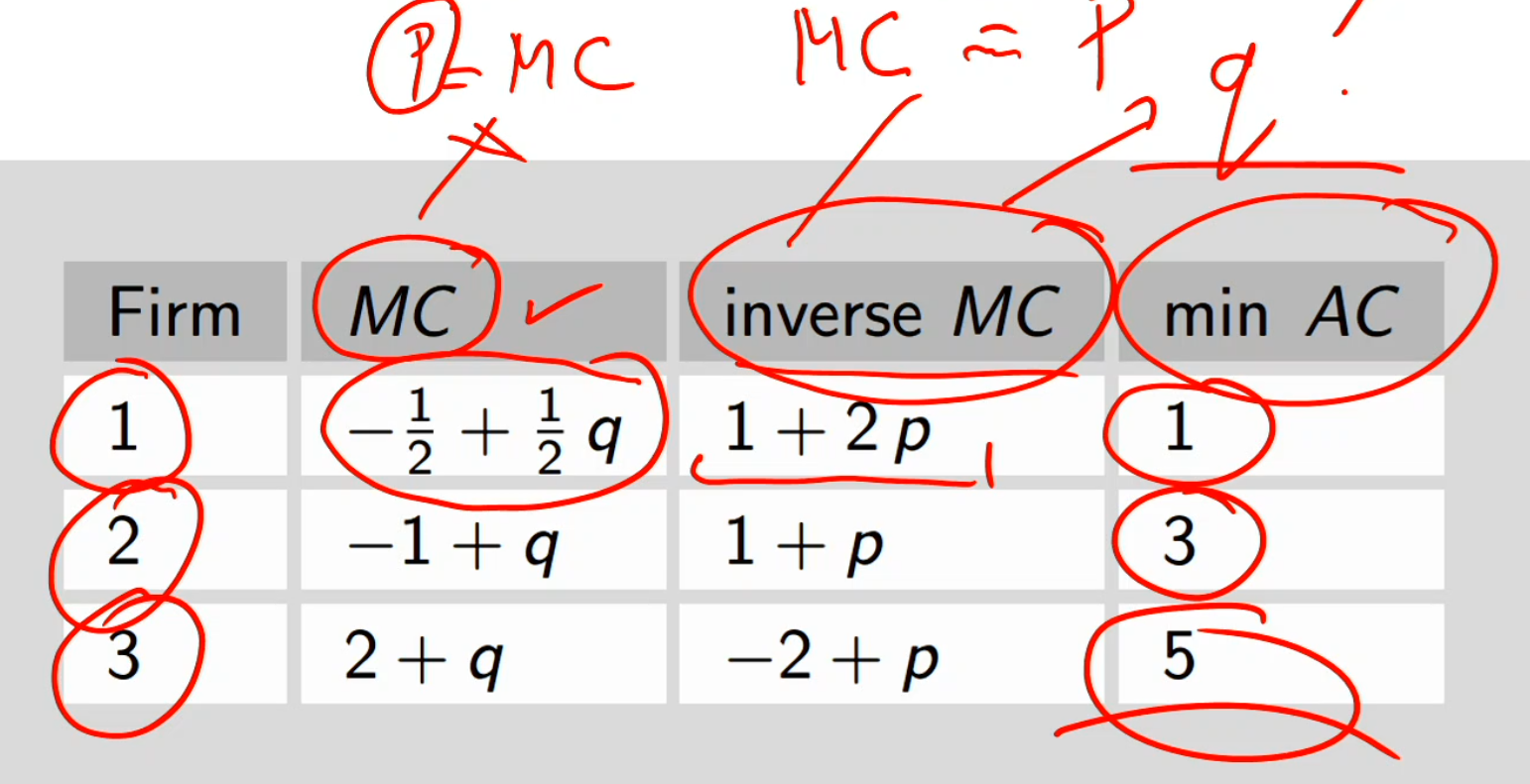
Firm supply to market supply

Firm 1 table:

MC

• p = mc

Inverse MC

• 1 + 2 = p came from switching to MC on the left and p on the left so mc = p

Min AC

• Firm 1 needs to give at least $1 minimum to produce a given level of output

• No firms in this market would produce output if they’re getting a price of less than one

Graph:

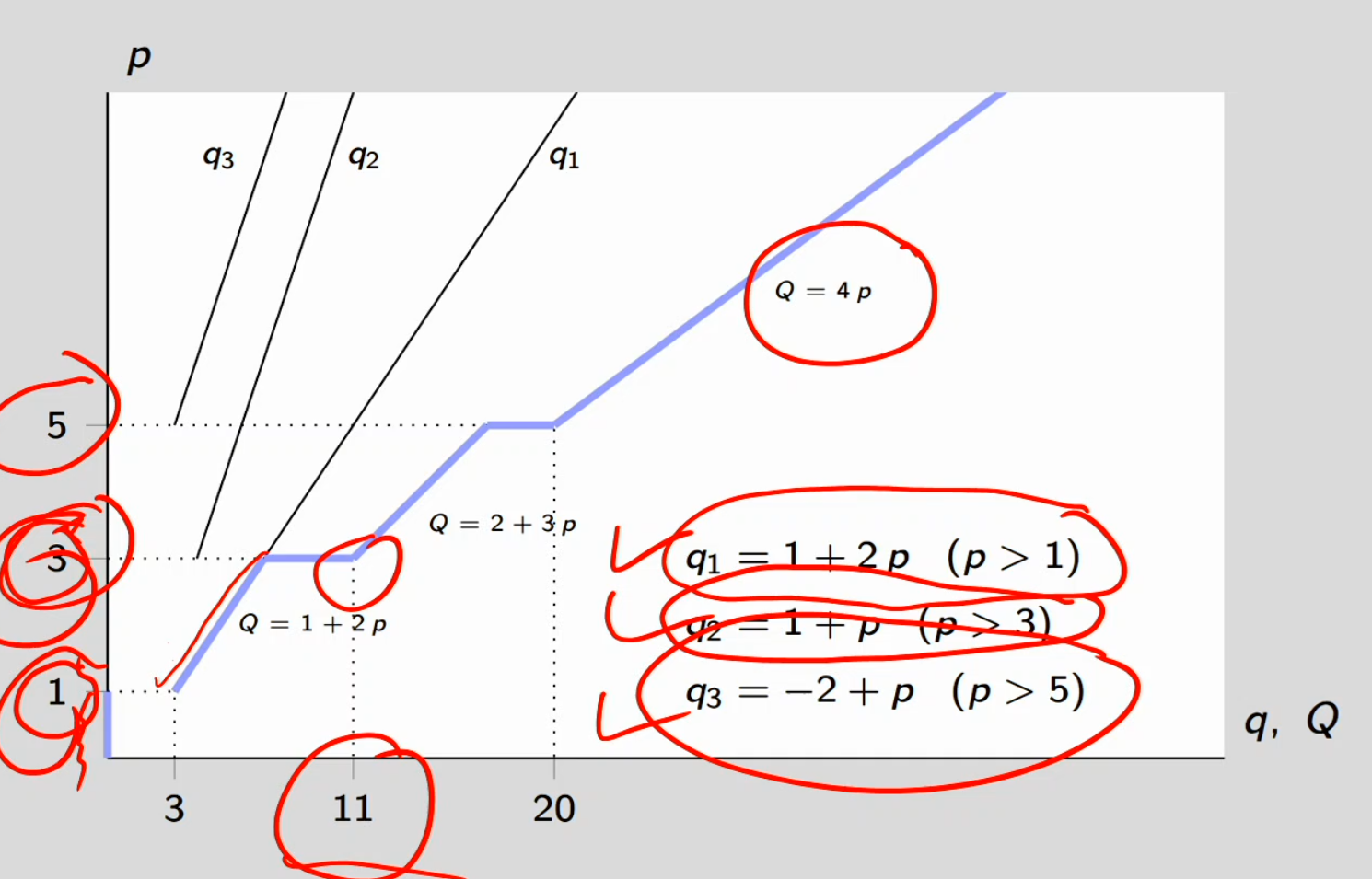
• Blue line is the market supply curve and it’s the horizontal summation of the individual supply curves in the market firms 1, 2, and 3

• Firms Enter at Different Prices:

  p < 1: No firms produce (all below min AC)

  • Q = 0

  1 ≤ p < 3: Only Firm 1 active

  • Q = q₁ = 1 + 2p

  3 ≤ p < 5: Firms 1 and 2 active

  • Q = q₁ + q₂ = (1 + 2p) + (-1 + p) = 2 + 3p

  p ≥ 5: All three firms active

  • Q = q₁ + q₂ + q₃ = (1 + 2p) + (-1 + p) + (-2 + p) = 4p

  Visual: Blue line with multiple segments, getting steeper as more firms enter

  Key Points on Graph:

  • At p = 1: Q = 3 (Firm 1 enters)

  • At p = 3: Q = 11 (Firm 2 enters, curve gets steeper)

  • At p = 5: Q = 20 (Firm 3 enters, curve gets even steeper)

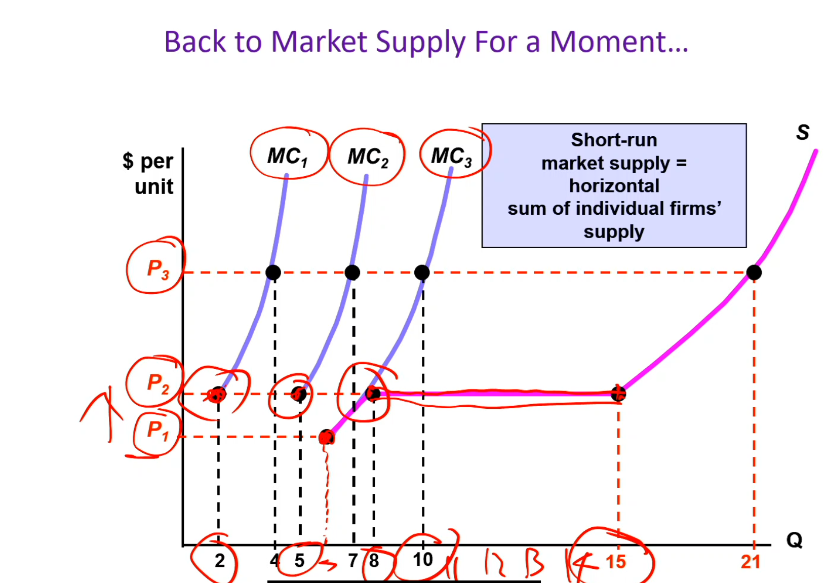
Market supply

At p1

• Only firm three is willing to step up 

At p2 

• All three firms are willing to step up

• 2 + 5 + 8 = 15, which is revealed by 15 by the purple market supply. We’re supplying UP TO 15 units of output (15 and less), therefore, it’s horizontal.

At p3

• All three firms are willing to step up

Demand curve and function

• Consumer’s optimal choice, determined by MRS = MRT, leads to x* and y* given px , py , and I (and given consumer preferences)

• Different values of px lead to different values of x

• Demand curve (or direct demand curve): gives the quantity demanded for a given price

• Inverse demand curve: for a given quantity, gives the corresponding price. This dollar value is also referred to as willingness to pay.

• Demand function: in addition to price, includes other factors influencing quantity demanded (e.g., income, other prices

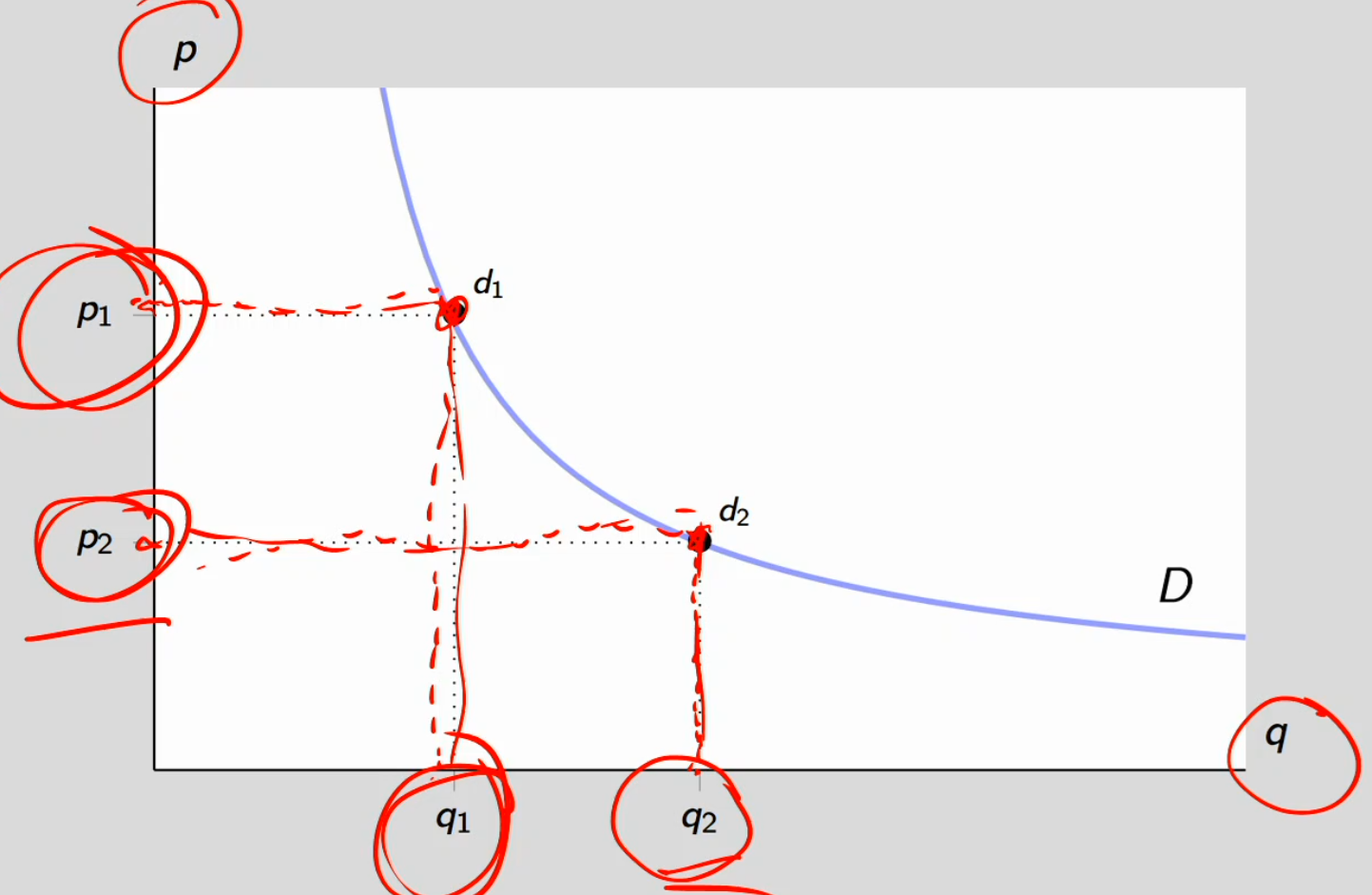
Demand curve

For a given quantity, what’s the price the costumers want to pay?

• If p = p1, then consumer purchases q1 units (direct demand)

• Also, p1 is the consumer’s willingness to pay for a q1th unit

• Demand curve is normally downward-sloping

• dThis property is normally referred to as the law of demand

From individual to market demand

Market Demand: Horizontal sum of all individual demand curves

Why Market Demand is Downward-Sloping

Two Reasons:

1. Intensive Margin: Existing consumers demand more as price falls

• Each individual's demand curve slopes down

• Lower p → each person buys more

2. Extensive Margin: New consumers "enter" market as price falls

• At high prices: only some consumers participate

• As price drops: more consumers find it worthwhile

• Similar to how firms enter supply market as price rises

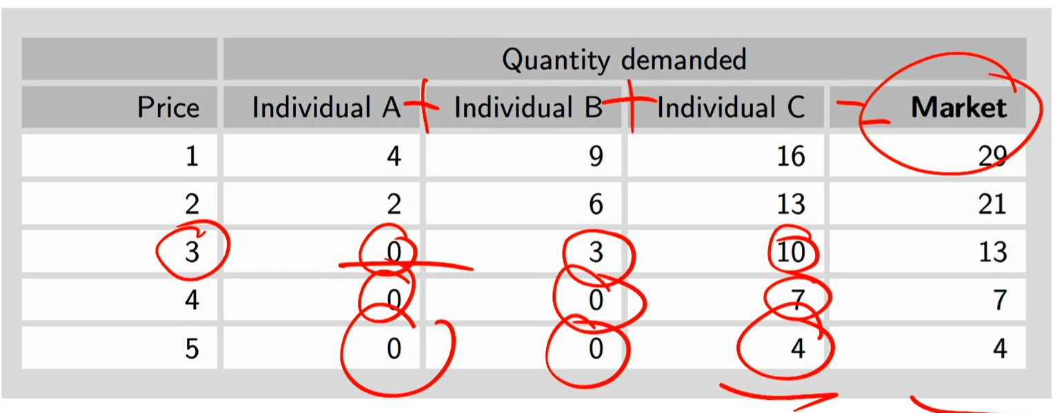
Market demand is obtained from individual demands in the same way as market supply is obtained from individual supply curves: by adding them “horizontally”, that is, adding qs for a given p.

At price 3:

• Individual B takes 3 units while individual C takes 10 units, the market equals to 13 units

• As price gets higher, we go from 3 to 4, individual B drops out so there only remains individual C with the market at 7

Demand for minivans

• Goal: estimate demand for minivans for each of the 50 US states

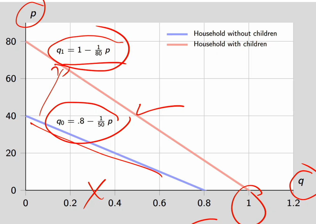
• Suppose the demand for minivans for a typical US household depends on whether the household includes children under 18 (q1) or not (q0).

  • q0 = .8 - 1/50p

  • q1 = 1 - 1/80p

• Each state has a given # households with children and a given # households without children. Aggregating over households, we get total demand at state level.

• For simplicity, in what follows assume US consists of two states, New Mexico (NM) and West Virginia (WV)

Inverted the function, put the p on the left and q on the right

• Red line:

  • If you plug in 0 for p, then q is 1

  • If you plug in 0 for q, then p is 80

  • Demand is higher for the red line (household with children) as willingness to pay for vans is higher

Market demand for minivans

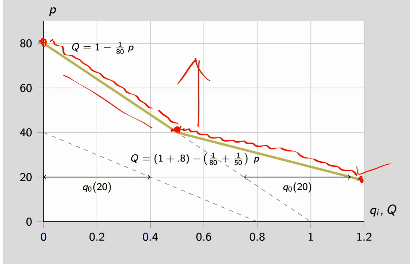
• Suppose, for simplicity, that there is one household with children and one household without children

• Then market demand, Q, is simply horizontal sum of the two household demand curves

• As price decreases, market demand increases for two reasons:

  • (a) individual buyers increase demand

  • (b) more buyers “enter” the market

Graph: market demand for minivans

• At price of 40 and above, the household with kids is more willing to buy vans (the line to the left) whereas below 40, belongs to the household with no kids. The entire line represents the horizontal summations of both households.

  • Exists a kink at 40

Families and children, by state data

Qnm is the demand for NM

• Households with children is more than WV

• There’s a choke point of demand = 0 at price above $80

• Within the interval $40 < p <_ $80, the only people that are willing to step forward are the households with kids 

  • Multiply households with kids (235) by the equation

• For price less than $40, both households step forward

  • Multiply households with kid and without by equation

  • The equations are the demand curves

Qnm is the demand for WV

• P > $80, neither the households step forward so demand = 0

• At $40 < p <_ $80, only the households with kids step forward

• At $40 and less, both households step forward

• Sum these to get the market demands

Market demand for minivans

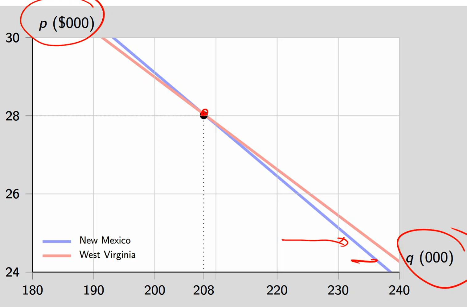
Assumed households with children in NM and WV are similar. However, market demand in NM is less sensitive to price than demand in WV. This is because there are more households with children in NM and households with children are less sensitive to price changes.

• They’re less sensitive to price changes because households in NM need minivans as necessities, not really any options for substitutes 

• The slope of NM is steeper, meaning it’s less sensitive to price changes

Surprising Finding: Despite WV having MORE households (504k vs. 467k), demand levels are similar

Explanation: NM has HIGHER percentage with children (50.4% vs. 42.3%)

• Type 1 households demand more minivans

• Higher child percentage offsets lower total households

At p = $28,000: Total demand is EXACTLY the same in both states

But Slopes Differ:

• NM demand: STEEPER (less price-sensitive)

• WV demand: FLATTER (more price-sensitive)

Why? NM has more families with children → more "dependent" on minivans → less willing to substitute away when price rises

Inverse demand curve

Inverse Demand D⁻¹(q): For a given quantity q, gives the willingness to pay for that qth unit

Two Ways to Read Demand:

1. Direct Demand D(p):

• Given price p → what quantity demanded?

• Answer: q = D(p)

2. Inverse Demand D⁻¹(q):

• Given quantity q → what is willingness to pay for that unit?

• Answer: p = D⁻¹(q)

Key Insight: Since optimal behavior implies p = MRS = willingness to pay, inverse demand reveals willingness to pay for each unit

The market mechanism

• The law of supply and demand states that price tends to move in the direction of the equilibrium price (where supply equals demand)

• The pendulum analogy

• Just like gravity pulls a pendulum towards its rest point, market forces (buyers and sellers) push price toward its rest point (equilibrium price)

  • When we’re at disequilibrium (pendulum swinging), for market forces, the behavior of those buyers and sellers is going to push us towards the equilibrium price (resting point) through gravity as it eventually reaches the resting point

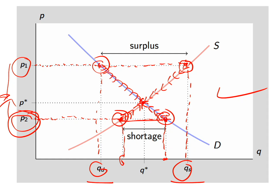
Graph:

• Equilibrium (resting point) at q* and p* where demand = supply

• At p1, the supply of qs is > the demand of qd, which is a disequilibrium at a surplus (excess supply)

  • There’s a downward pressure on price

  • In response to downward pressure on price, consumers will react with an increase in quantity demanded and the producers will respond to a decrease in quantity supply

  • We’re going to move down along the demand curve, no shifting just move along

  • We’re also going to move down along the supply curve

  • Now the pendulum reaches the resting point at p*, the equilibrium

• At p2, the demand of qd is > the supply of qs, which is a disequilibrium at a shortage (excess demand)

  • There’s an upward pressure on price

  • In response, producer will move up the supply curve as producers have an incentive to produce more output

  • Move up along the demand curve

  • Now back at equilibrium

Comparative statics 

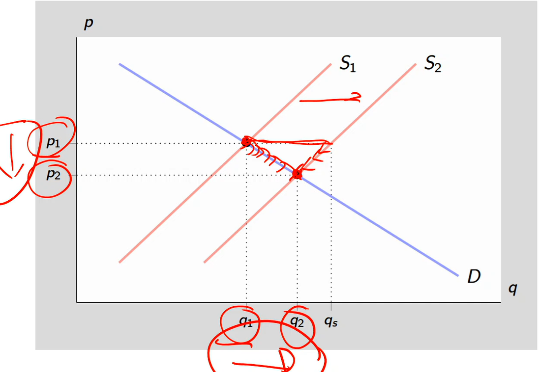
• A rightward shift of the supply curve leads to an increase in quantity and a decrease in price

  • S1 shifts right to S2

  • For any given price, you could now supply more output because your cost of production is going down

  • At p1 is disequilibrium, so we shift to p2 with a downward pressure on prices

    • Move down and along the demand curve, so quantity demand will increase

    • Move down and along the supply curve, so quantity supply will go down

  • q1 moves to q2

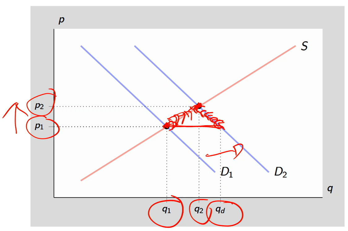
• A rightward shift of the demand curve leads to an increase in quantity and an increase in price

  • D1 shifts right to D2

  • There’s now disequilibrium because there’s a gap between q1 and qd

  • There’s an upward pressure on prices

  • Quantity supply will go up whole quantity demanded will go down

  • Back at equilibrium as the pendulum stops

  • As a result of the rightward shift, we ended up with a higher equilibrium price and quantity so p and q are both higher

Shift versus movement along of supply curve

Movements along the supply curve of x, while other factors remain the same, correspond to changes in the price of x

Shifts in the supply curve of x result from changes in factors other than the price of x

• Cost of production

• Geological shock/natural disaster that hits natural resources

• Technology

• Availability of workers that affect the price of workers

• Number of suppliers

• Regulation, how does this affect supply?

Graph:

• S1 = S2

• Let’s say price of services goes up

• So supply curve goes up and along from E1 to E2 and q1 to q2

• The supply curve shifts to the right to E3 and Q3 from a sudden shock

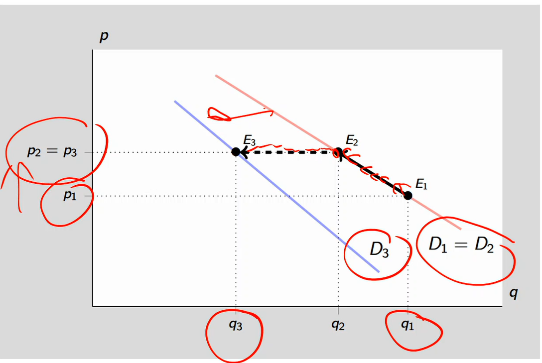
Shift versus movement along of demand curve

Movements along the demand curve of x, while other factors remain the same, correspond to changes in the price of x

Shifts in the demand curve of x result from changes in factors other than the price of x

• Change in income

• Change in the price of related goods

• Change in preferences/taste

• Product recalls

• Population changes/demographics 

  • Number of buyers/consumers

• Expectations

Graph:

• Raising the price leads to up and along the demand curve from E1 moving to E2

• The demand curve shifts leftwards/inwards

  • Due to reasons like decrease income

• Shifts to a new demand curve at D3

  • Demand is now lower

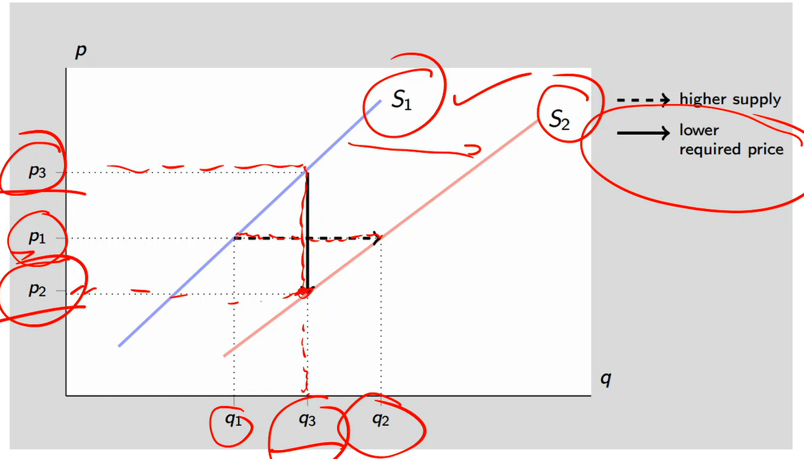
Supply shift

Starting at p1 and q1

• Higher supply arrow: Supply curve shifts from S1 to S2 so q1 becomes q2

  • Higher supply due to reasons like loosened regulations, productivity shock, etc

• Lower required price arrow:

  • The firm required a price of p3 to bring that unit to market. If you ask them, I’m considering supplying q3 units of output, what’s the minimum price you require?

  • Post supply curve shift from S1 to S2

    • For a given level of output, what’s the minimum price you must give me as a firm to bring that unit to market?

    • The price you need (p2) is lower than the price you need pre-shift of p3

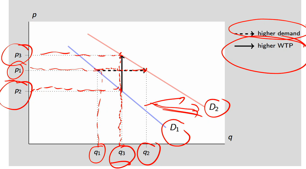
Demand shift

Starting at p1 and q1

Higher demand arrow:

• There’s an increase in the price of a substitute good

• Rightward shift of the curve, higher demand 

Higher WTP (willingness to pay) arrow:

• Let’s see if the new demand curve of D2 wants to pay for that same good or service 

• Willingness to pay has changed and is higher because the demand curve is now greater

Effects on p and on q

The more sensitive supply is to changes in price, the more the effect of a demand shift will be felt on output as opposed to price

The more sensitive demand is to changes in price, the more the effect of a supply shift will be felt on output as opposed to price

Top left:

• Supply curve is much flatter compared to demand curve

• Demand shifts from D1 to D2

• The impact is mostly felt on Q compared to P

Top right:

• Supply curve is much more steep than demand curve

• Demand shifts from D1 to D2

• The impact is mostly felt on P than Q

Bottom left:

• The demand curve is much more flatter than the supply curve

• Supply shifts from S1 to S2

• The impact is mostly felt on Q than P

Bottom right:

• The demand curve is much more steeper than the demand curve

• Supply shifts from S1 to S2

• The impact is mostly felt on P than Q

First theorem of welfare economics

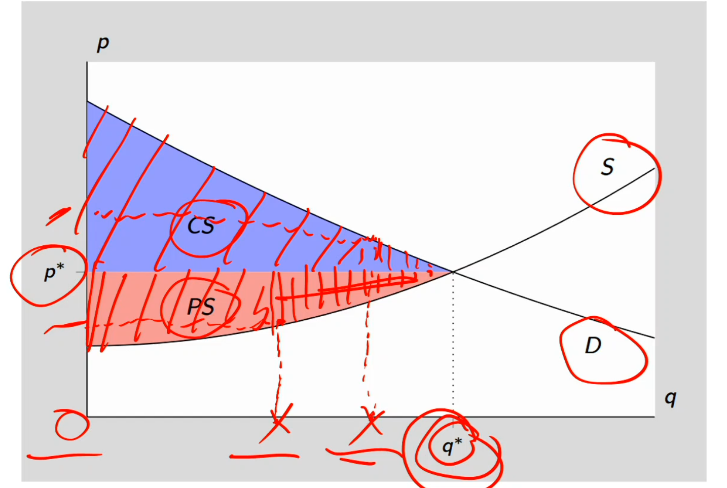
First theorem of welfare economics: in a competitive market, the equilibrium levels of output and price correspond to the maximum total surplus

• The market, on its own, chooses the price and quantity that create the greatest benefit for society (buyers + sellers combined

Consumer surplus: the difference between how much consumers are willing to pay and how much they actually pay (p*)

Ex: between 0 and $10, for that particular unit, their willingness to pay is greater than the price they actually paid

• Some buyers would have paid $10

• But price is only $6

• They "save" $4 → that’s surplus

• So they’re earning the area of he consumer surplus as their willingness to pay is greater than the price you actually have to pay at p*

Producer surplus: difference between the price sellers receive AKA the market price (p*) and the minimum they require to produce each unit (cost of producing goods)

• For early units, cost might be $2

• Market price is $6

• Seller earns $4 profit-like benefit → producer surplus

• At equilibrium q*, consumer surplus and producer surplus are both maximized

  • welfare, efficiency, are maximized