logistic regression

generative classifiers + discriminative

if distinguishing cat from dog images = generative classifier

build a model of what’s in a cat image

• whiskers, eyes ears

• assigns prob to any image to determine how cat-like is that image?

• similarly, build model of what’s in dog image

now given new image, run both + see which fits better

If we are distinguishing cat from dog images using a Discriminative Classifier.

• Just try to distinguish dogs from cats. Oh look, dogs have collars. - Let’s ignore everything else.

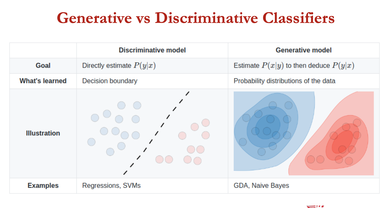
generative vs discriminative classifiers

generative (naive bayes)

• assume some form of conditional independence

• estimate parameters of P(D|h), P(h) directly from training data

• use bayes rule to calculate P(h|D)

why not learn P(h|D) or decision boundary directly?

discriminative (logistic regression)

• assume some functional form for P(h|D) or for the decision boundary

• estimate parameters of P(h|D) directly from training data

Naïve Bayes:

• 𝑌_𝑁𝐵=𝑎𝑟𝑔𝑚𝑎𝑥_h𝑃(𝐷|h) ⋅𝑃(h)

logistic regression:
- 𝑌_𝐿𝑅 = 𝑎𝑟𝑔𝑚𝑎𝑥_h𝑃(𝐷|h)

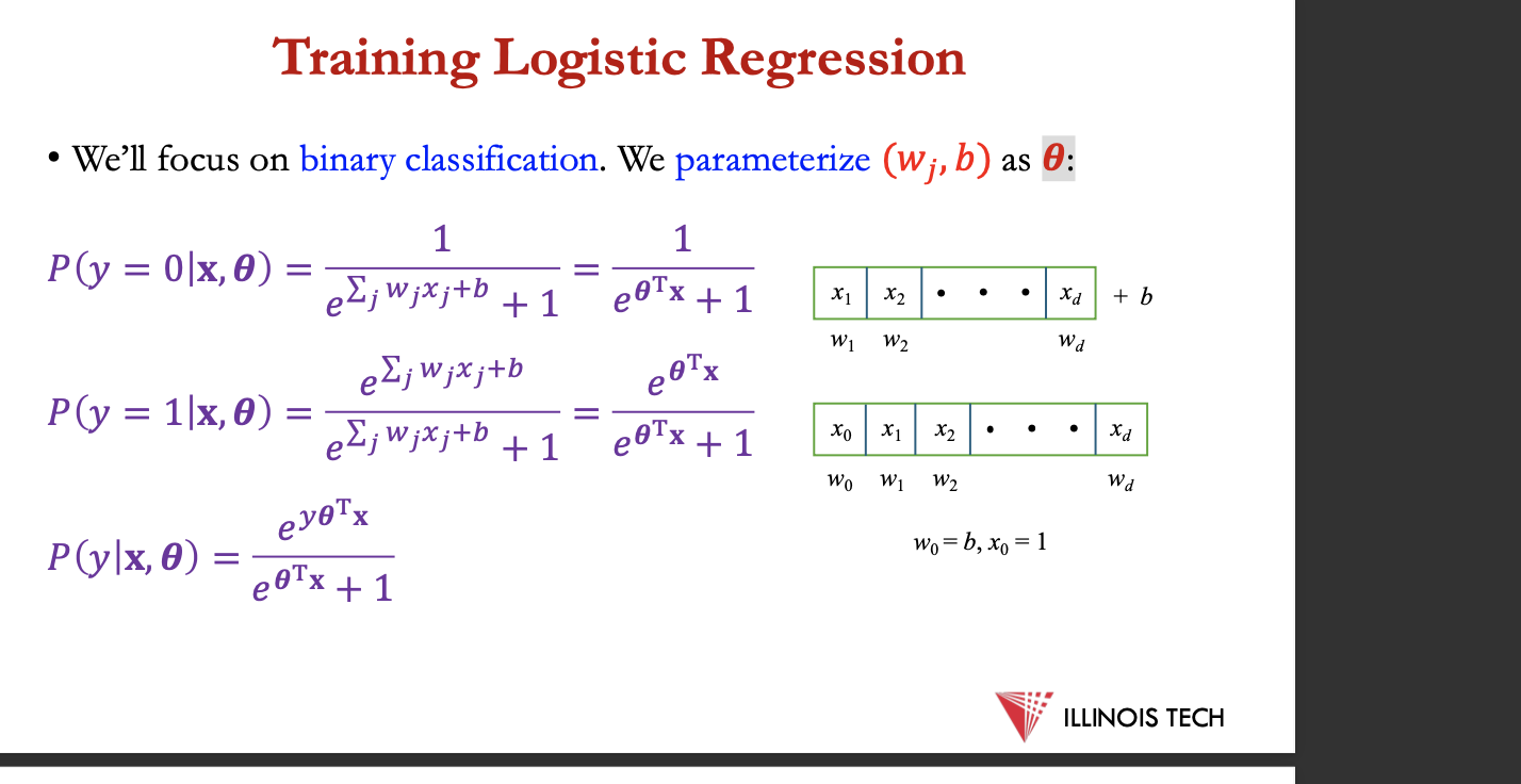
learning a LR classifier

given n input-output pairs:

1. a feature representation of the input. For each input observation x, a vector of features [x1, x2, …, xd]

2. a classification function that computes y, the estimated class via P(y|x), using the sigmoid or softmax functions

3. an objective function for learning, e.g. cross-entropy loss

4. an algo for optimising the objective function - stochastic gradient ascent/descent

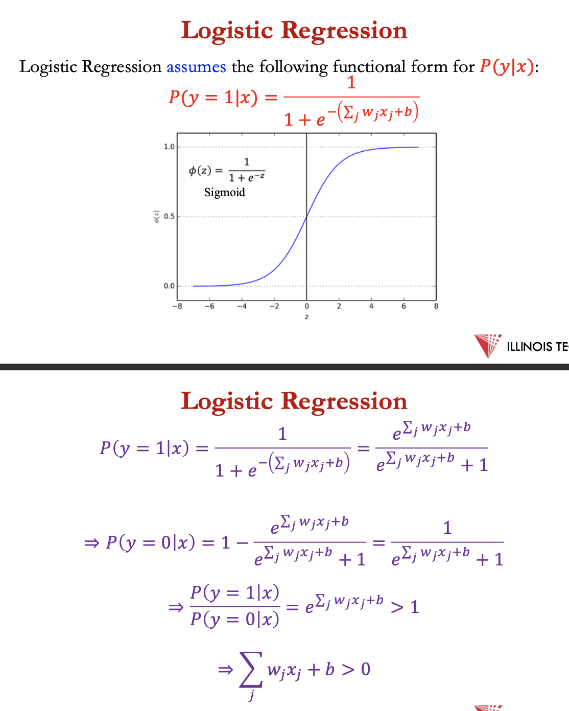
LR

LR assumes the following functional form for P(y|x):

P(y=1|x) = 1/ (1+e ^ (-(∑ j wjxj +b)))

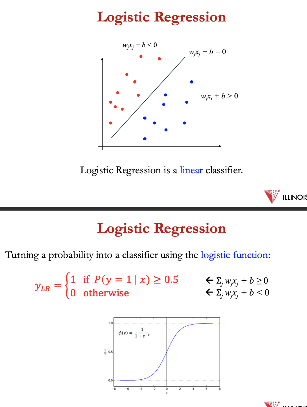
→ ∑ wjxj + b > 0

logistic regression = linear classifier

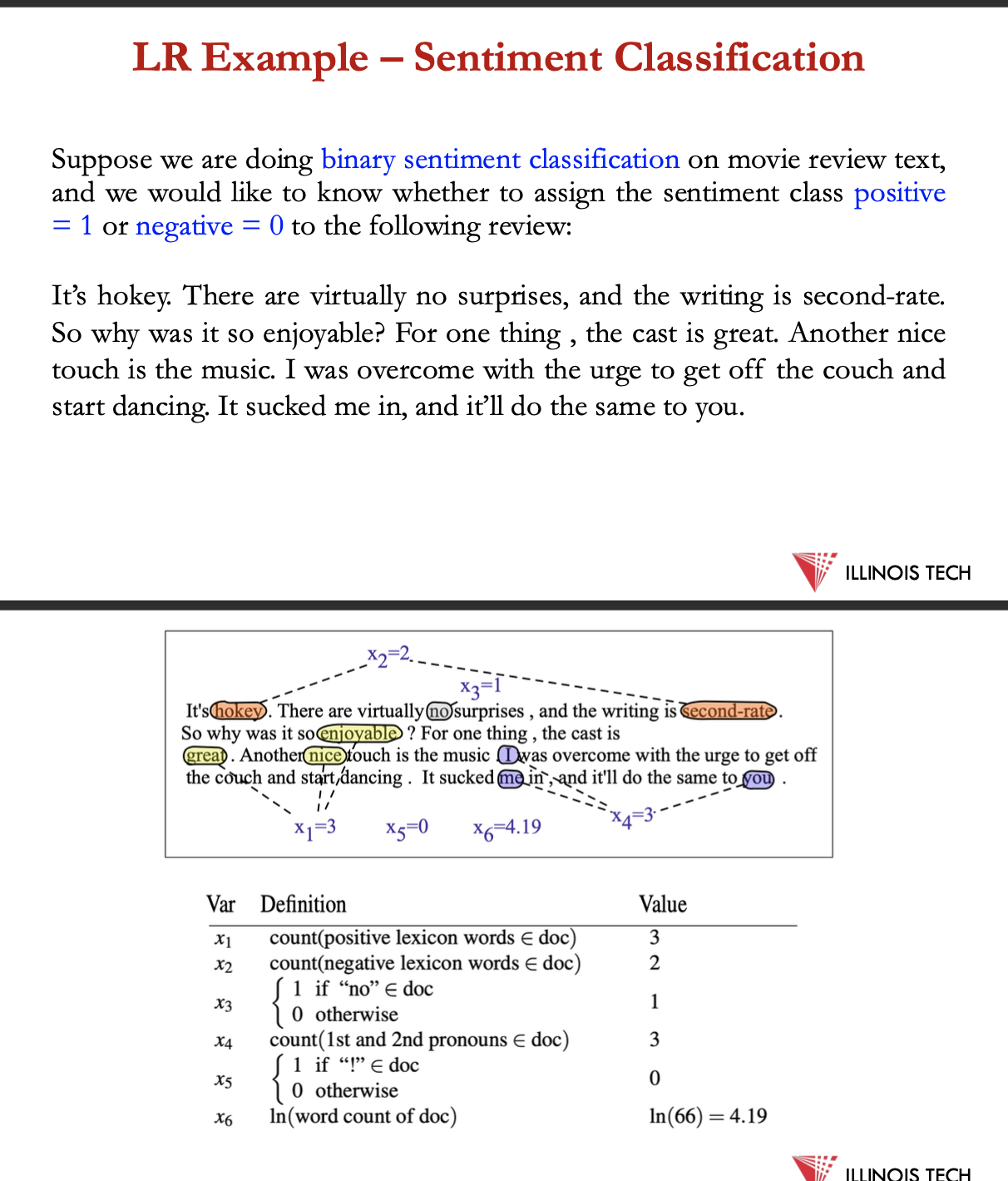
LR example - sentiment classification

e.g. doing binary sentiment classification on movie review test + we’d like to know whether to assign the sentiment class +ve = 1 or -ve = 0 to the following review:

Let’s assume for the moment that we’ve already learned a real-valued weight for each of these features, and that the 6 weights corresponding to the 6 features are [2.5, −5.0, −1.2, 0.5, 2.0, 0.7], while b = 0.1.

training LR

we’ll focus on binary classification

• we parameterise (wj,b) as 𝜽:

p(y| x, 𝜽) = e^y𝜽Tx/ e^𝜽Tx + 1

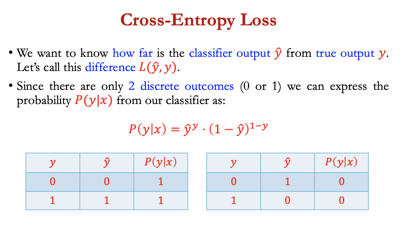
cross entropy loss

want to know how far is classifier output ŷ from true output y , difference = L(ŷ,y)

2 discrete outcomes, can express probability

• P(y|x) = ŷ^y * (1-ŷ)^1-y

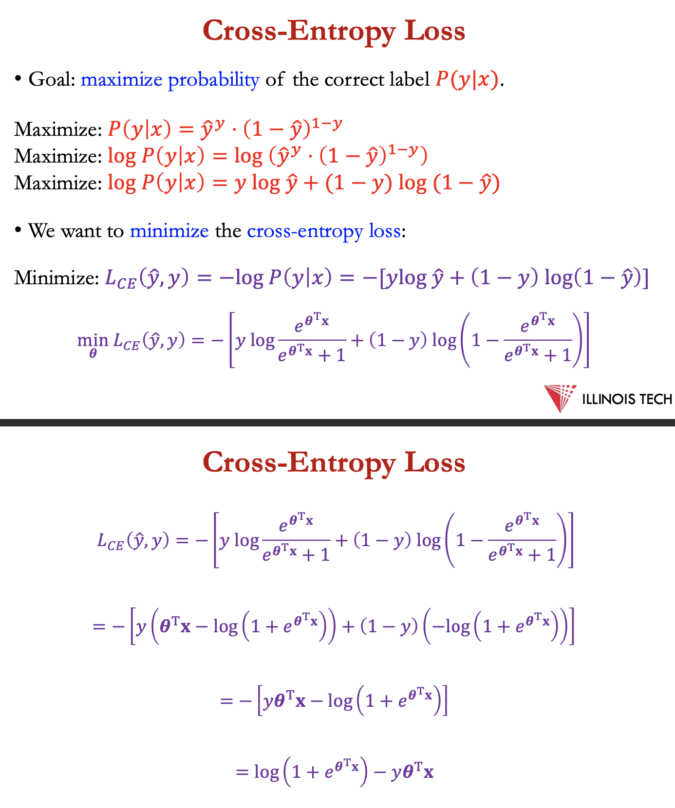
goal: maximise prob of the correct label P(y|x)

Maximize: P(y|x) = ŷ^y * (1-ŷ)^1-y

Maximize: logP(y|x) =log ( ŷ^y * (1-ŷ)^1-y)

Maximize: logP(y|x) = y log ŷ + (1-y)log (1-ŷ)

• want to min. cross entropy loss

= log ( 1+𝑒^𝜽T𝐱) −𝑦𝜽^T𝐱

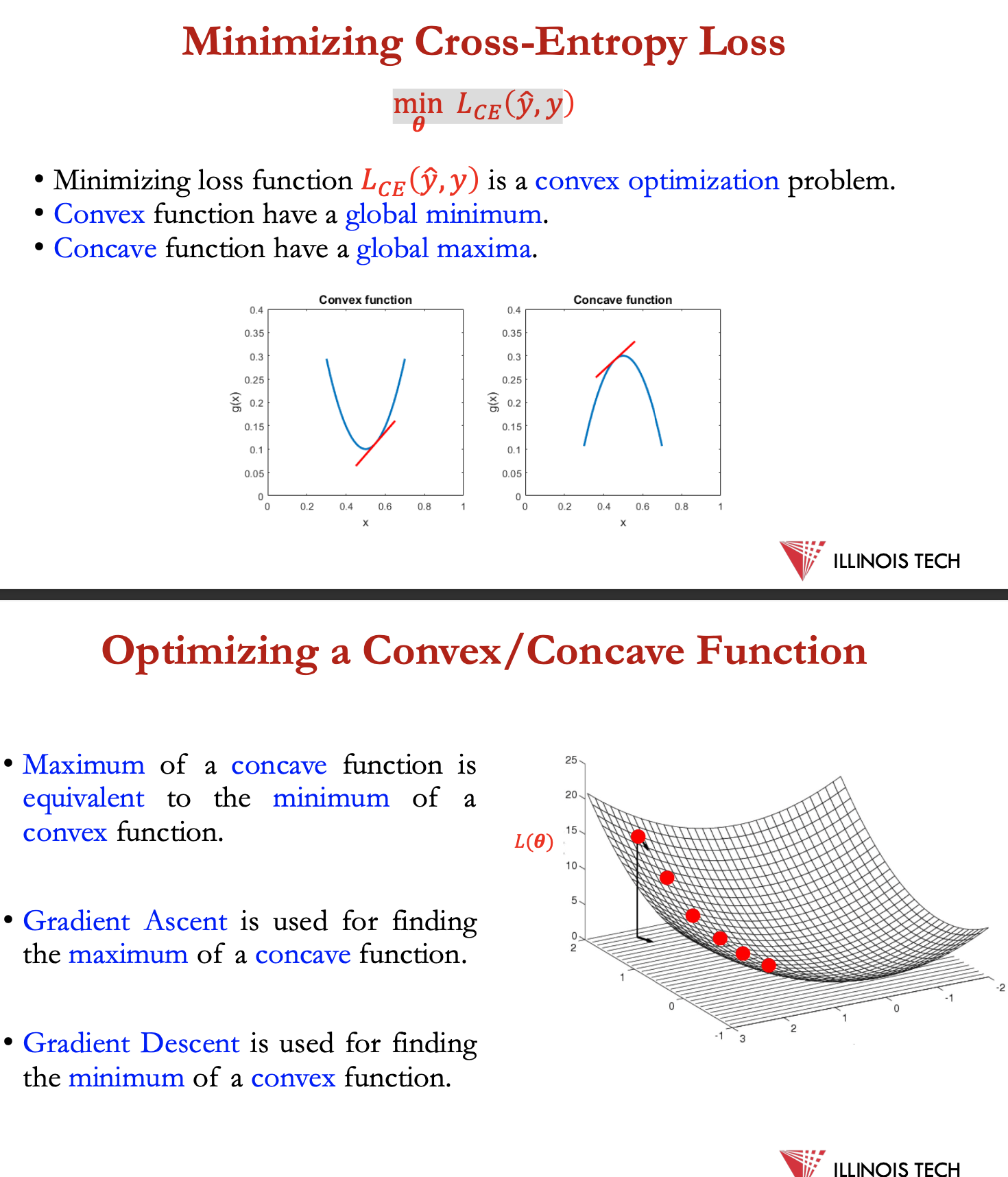
minimising cross entropy loss

min 𝐿 _{𝐶 𝐸} (ŷ,y)

• minimising above = convex optimisation problem

• convex function = global min → Gradient Ascent

• concave func = global max → Gradient descent

gradients:

• gradient of function = vector pointing in direction of the greatest increase in a function

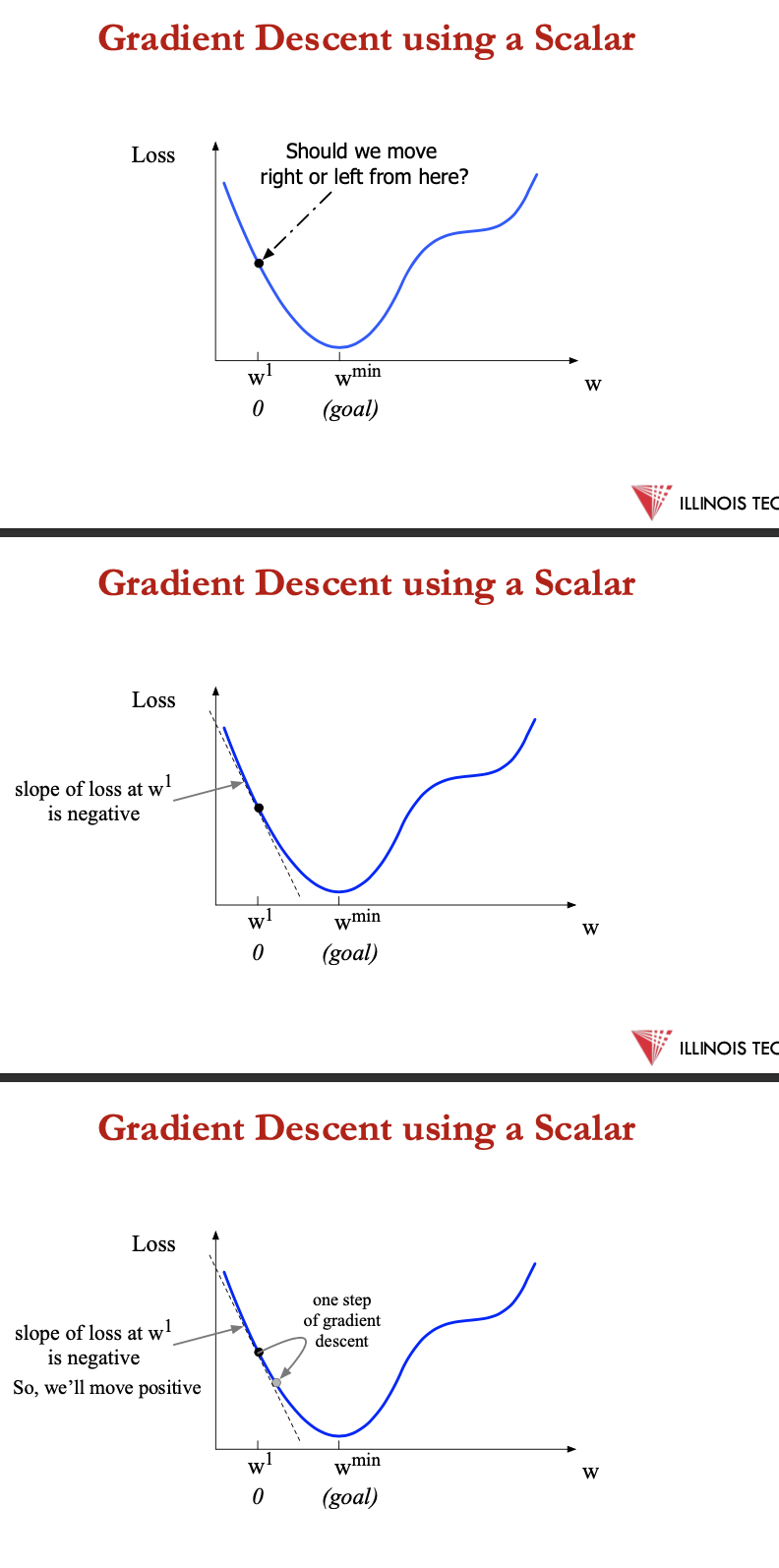
• Gradient Ascent: Find the gradient of the function at the current point and move in the same direction.

  • Gradient Descent: Find the gradient of the function at the current point and move in the opposite direction.

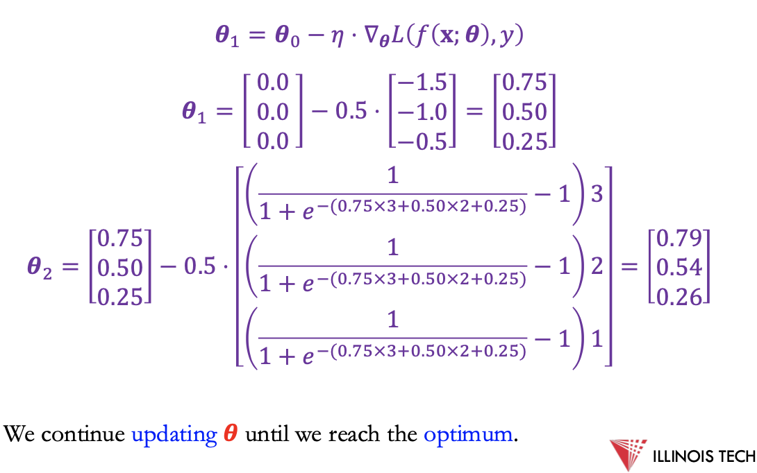
gd for LR

• Let us represent ŷ = 𝑓(𝐱; 𝜽)

𝜽_t+1 = 𝜽_t - 𝜂 ⋅ 𝐱 [1 / 1+ 𝑒^−𝜽T𝐱 - y]

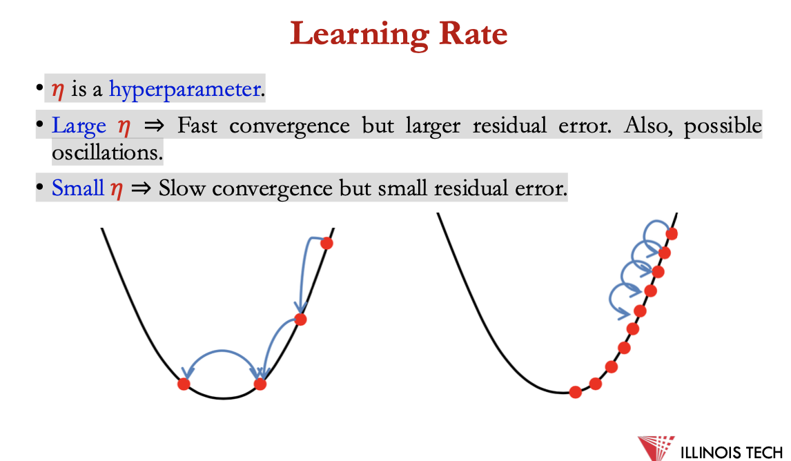
learning rate

𝜂 is a hyperparameter.
• Large 𝜂 ⇒ Fast convergence but larger residual error. Also, possible

oscillations.
• Small 𝜂 ⇒ Slow convergence but small residual error.

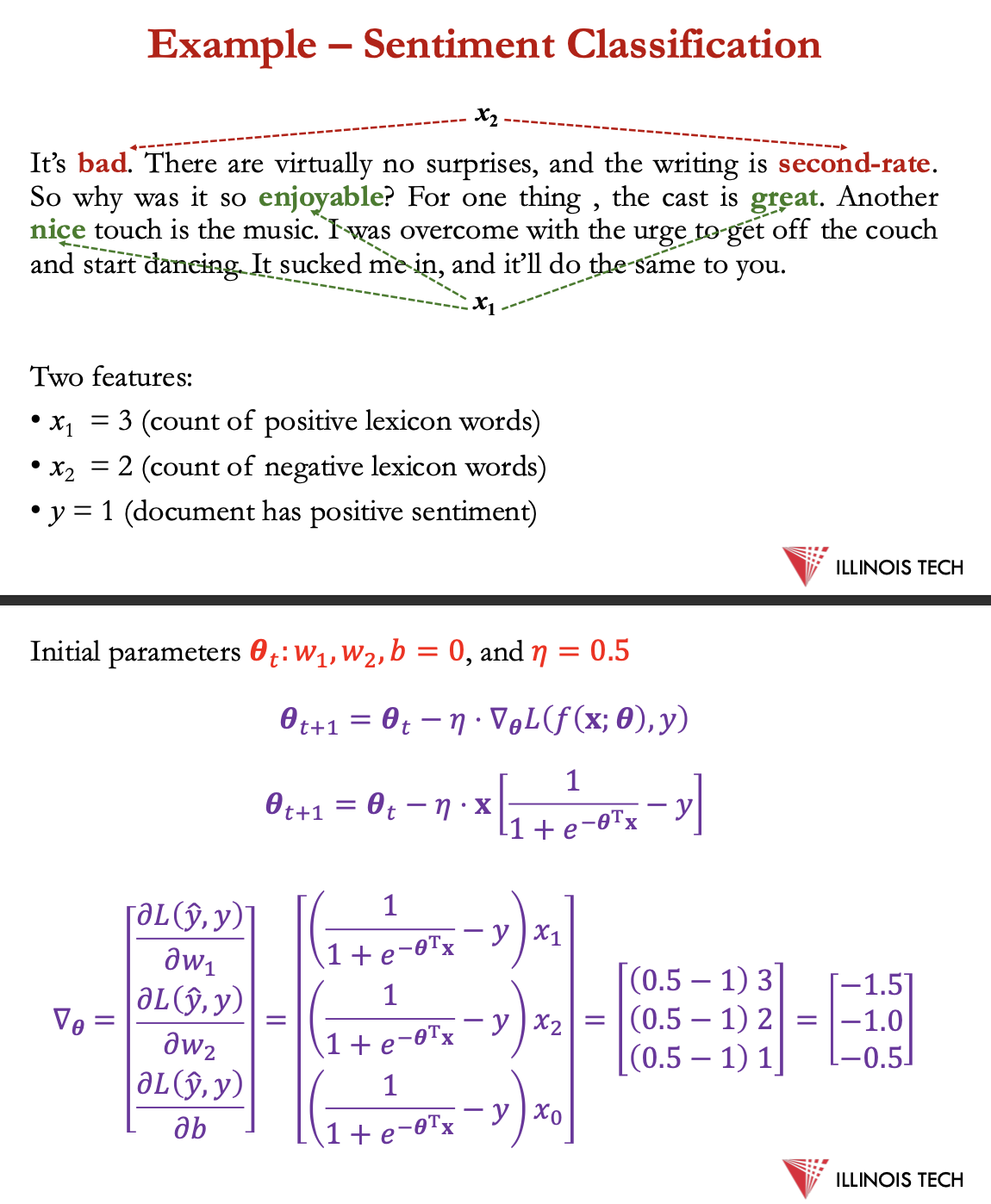
Example – Sentiment Classification

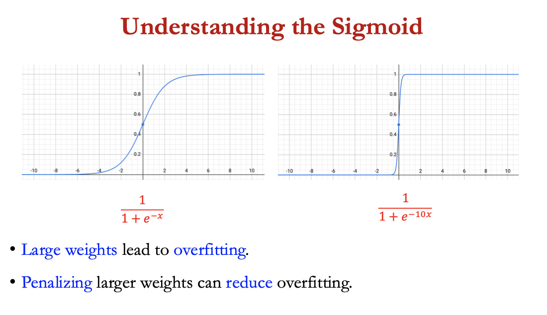
understanding the sigmoid

large weights = overfitting

penalising larger weights can reduce overfitting

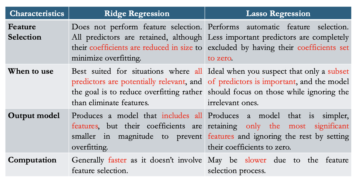
regularisation

used to avoid overfitting

weights for features will attempt to perfectly fit details of the training set, modelling even noisy data that just accidentally correlate with the class = overfitting

good model = generalises well from the training data to the unseen test set, but model that overfits will have poor generalisation

avoid overfitting = add regularisation term 𝑅(𝜽) to the loss function

min 𝐿_𝑟𝑒𝑔 (ŷ,y) =min (log (1+𝑒^𝜽T𝐱) −𝑦𝜽^T𝐱+𝜆𝑅 (𝜽))

more regularisation

L2 regularisation → ridge regression

• uses square of the L2 (euclidean) norm of the weight values

𝑅 (𝜽) = ||𝜽 ||₂² = ∑𝜽²_j

min 𝐿_𝑟𝑒𝑔 (ŷ,y) =min (log (1+𝑒^𝜽T𝐱) −𝑦𝜽^T𝐱+𝜆∑𝜽²_j )

L1 regularisation → lasso regression

• uses L1 norm (Manhattan distance) of the weight values

𝑅 (𝜽) = ||𝜽 ||₁ = ∑|𝜽_j|

min 𝐿_𝑟𝑒𝑔 (ŷ,y) =min (log (1+𝑒^𝜽T𝐱) −𝑦𝜽^T𝐱+𝜆∑|𝜽_j|)

batch training

stochastic g.d. - chooses single random example at a time, moving the weights so as to improve performance on that single example

= choppy movements, common to compute the gradient over batches of training instances over a single instance

training data: {𝑥𝑖 ,𝑦𝑖} _{𝑖=1...𝑛} where, 𝑥𝑖 = (𝑥𝑖1 ,𝑥𝑖2 ,...𝑥𝑖𝑑), 𝑛 is the total instances in a batch and 𝑑 is the dimension of an instance

𝜽_𝑡+1=𝜽_𝑡−𝜂/ 𝑛⋅∑ 𝐱_𝑖𝑗 [ 1/ 1+𝑒^−𝜽T𝐱−𝑦𝑖]

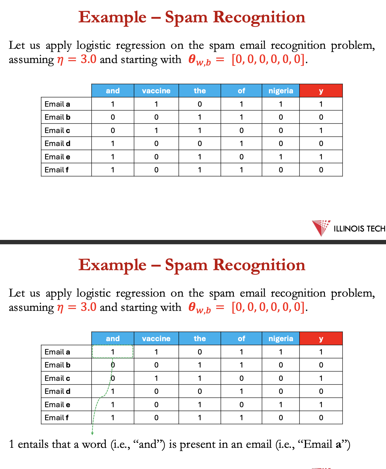
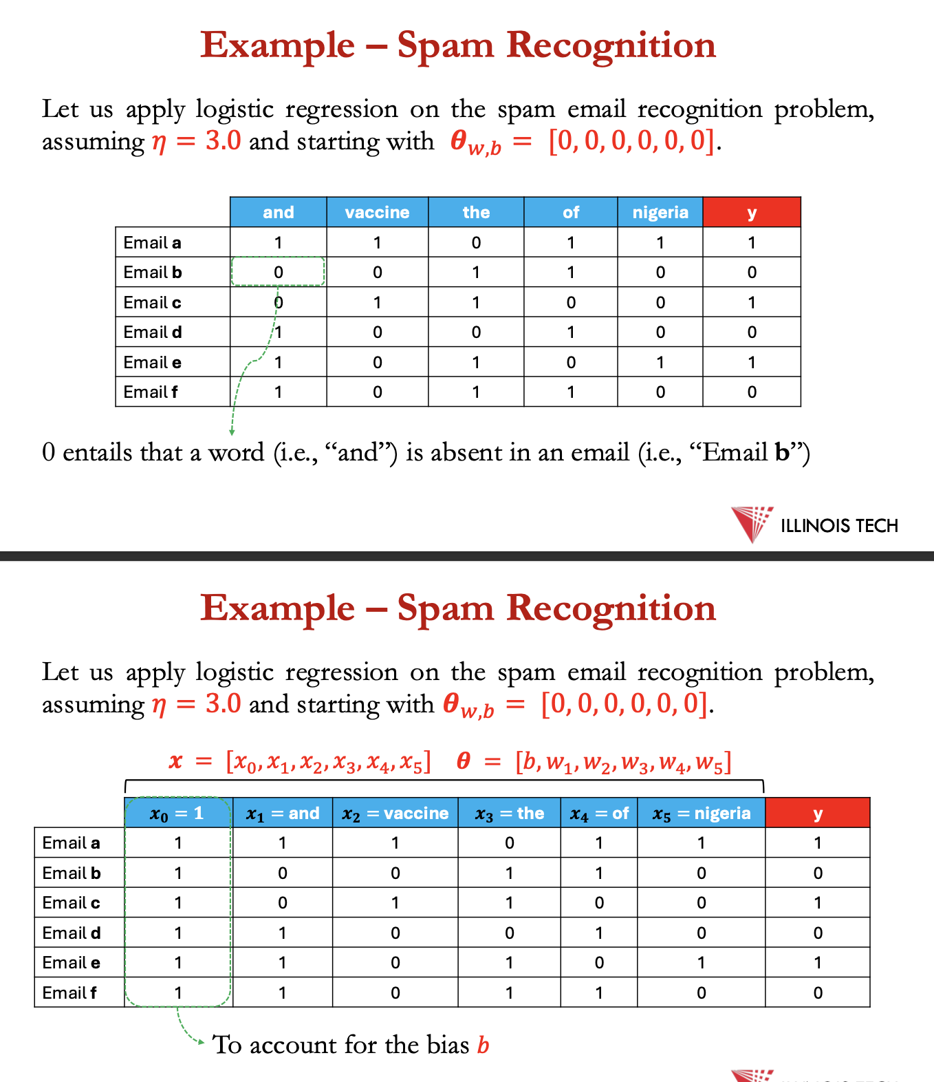
example - spam recognition

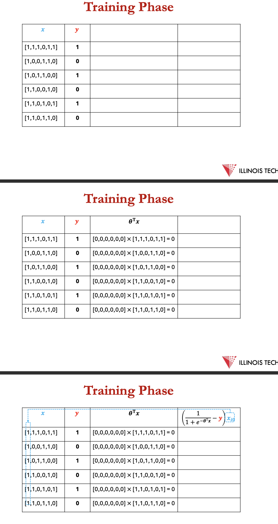
training phase

1st - calculate ^−𝜽T𝐱 for every example in the data set

2nd - calculate ∑ 𝐱_𝑖𝑗 [ 1/ 1+𝑒^−𝜽T𝐱−𝑦𝑖] for every example in data set for every 𝜽

3rd - compute every 𝜽_𝑡+1

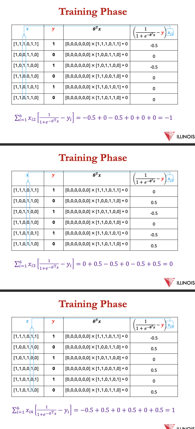
cont

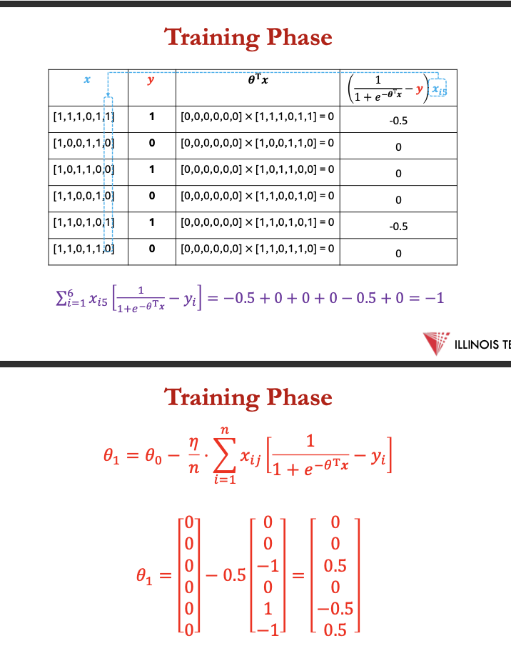
testing phase

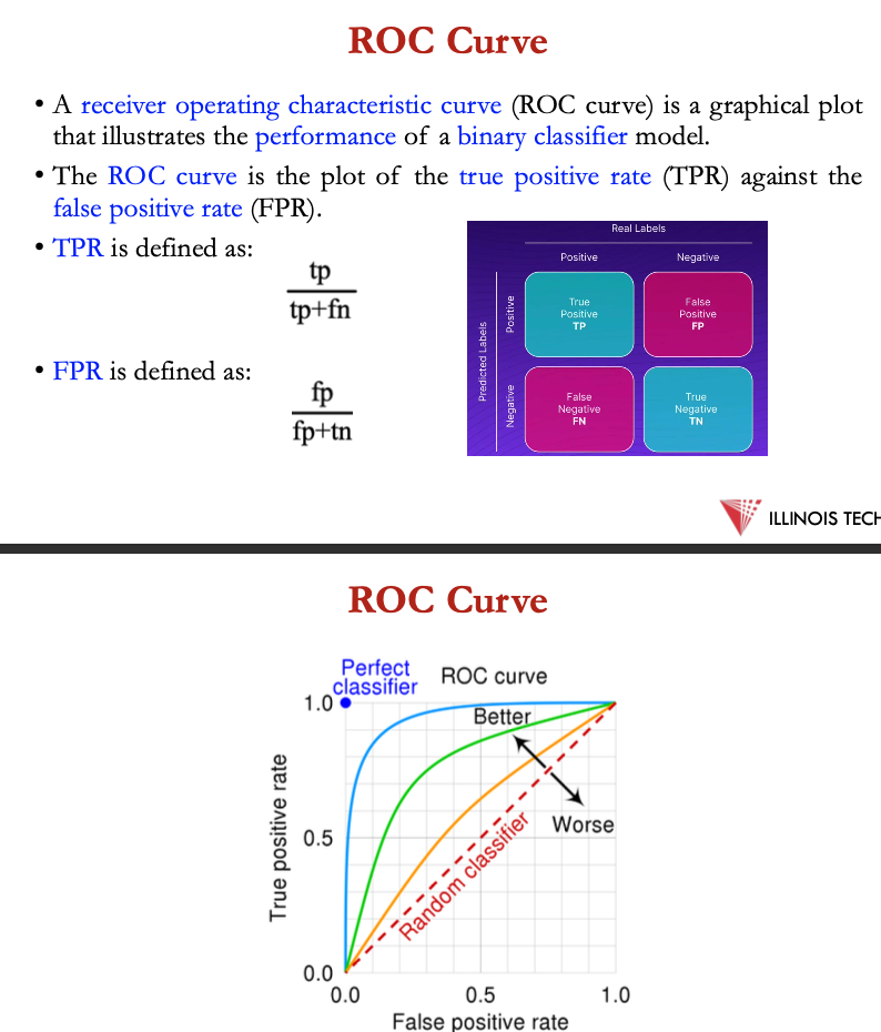
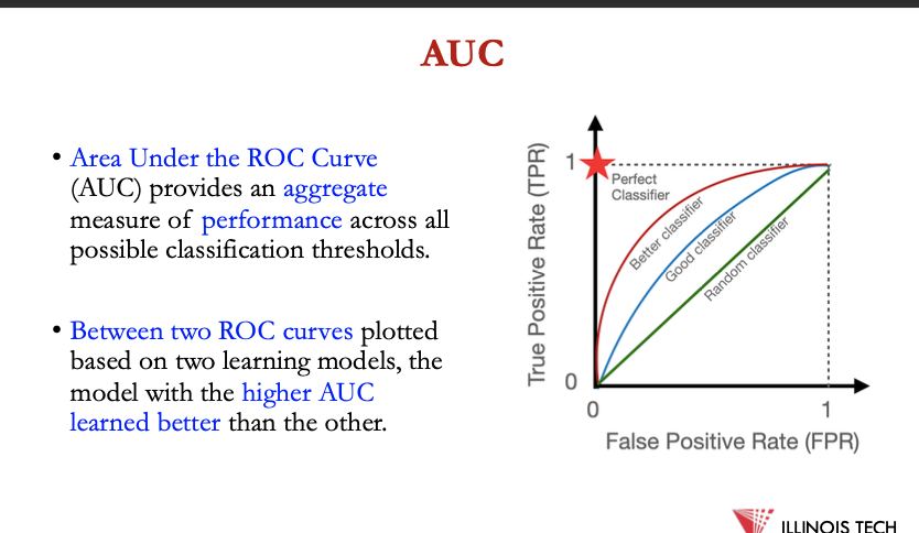
ROC curve

receiver operating characteristic curve = graphical plot that illustrates the performance of a binary classifier model

• ROC curve = plot of the true positive rate against the false positive rate

TPR:

• tp / (tp+fn)

FPR:

• fp/ (fp+tn)

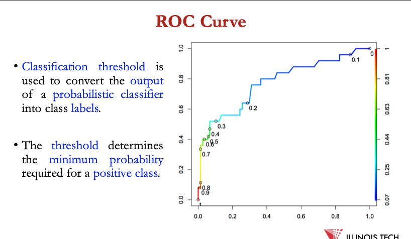
Classification threshold is used to convert the outputof a probabilistic classifier into class labels.

• The threshold determines the minimum probabilityrequired for a positive class

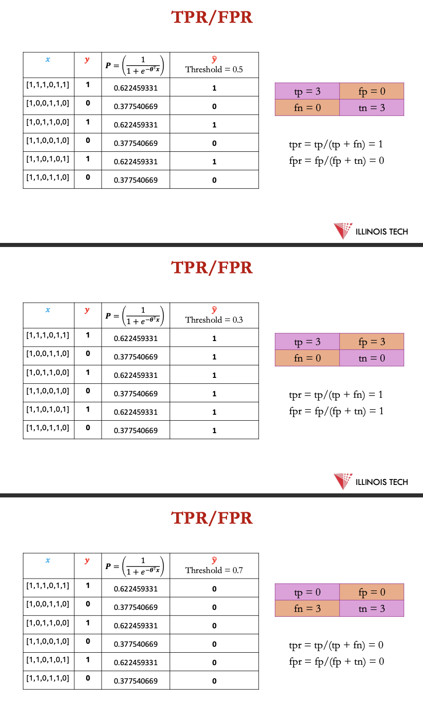
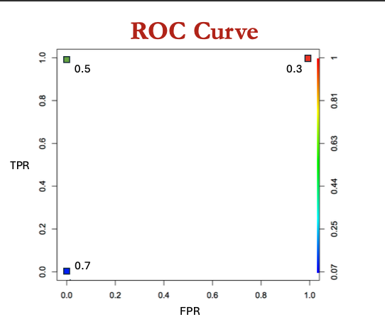
TPR/FPR

AUCa

area under the ROC curve provides aggregate measure of performance across all classification thresholds

between 2 ROC curves plotted based on 2 learning models, model w higher AUC learned better than the other

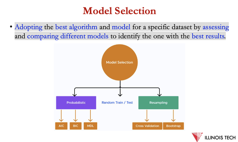
Model Selection

Adopting the best algorithm and model for a specific dataset by assessing and comparing different models to identify the one with the best results.

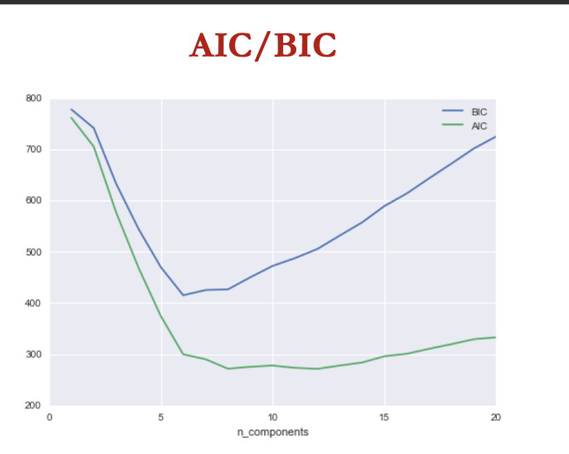
AIC/BIC

akaike info criterion + bayesian info criterion compares diff models to choose 1 that best fits the data

• goal of both AIC + BIC = balnce the goodness of fit of the model w its complexity in order to void overfitting or underfitting

both AIC + BIC penalises models w large no of parameters relative to size of data, but BIC penalises more severely

min 𝐴𝐼𝐶 = 2 𝑚 − 2 log 𝐿

min 𝐵𝐼𝐶 = 𝑚 log 𝑛 − 2 log 𝐿

• where m = no of model parameters, n = no of data points + L = max likelihood of the model

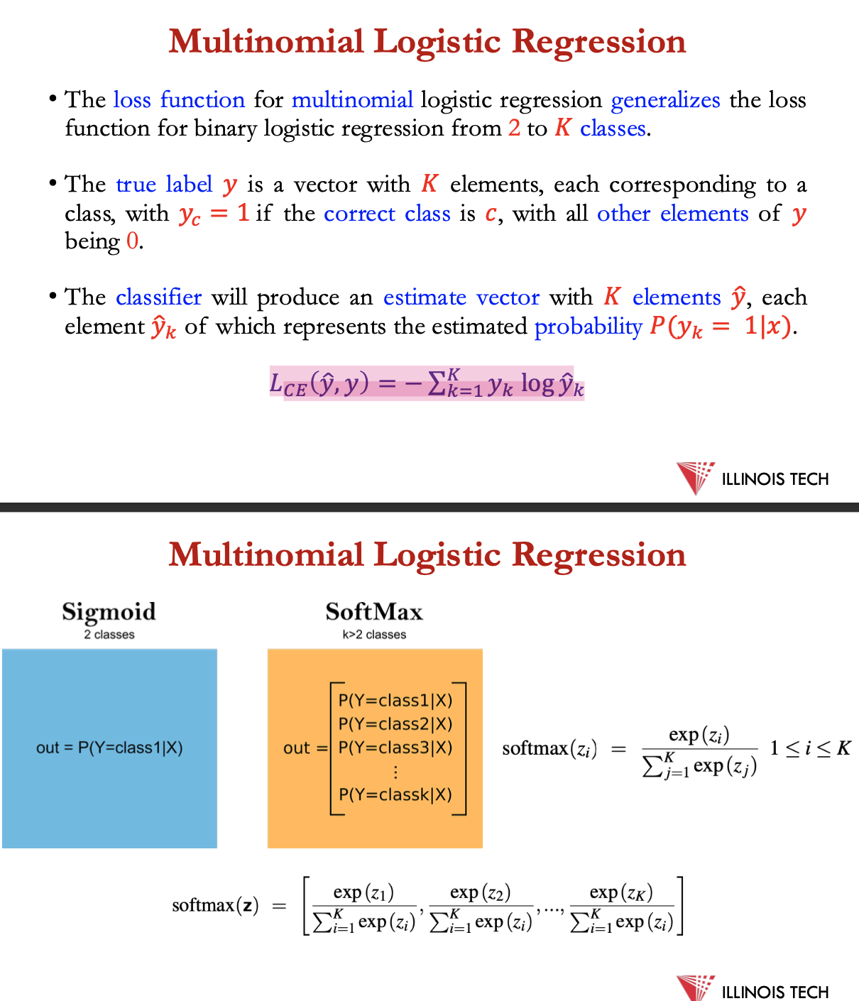
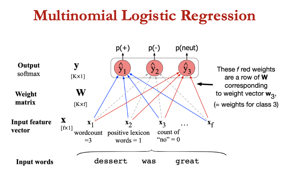
Multinomial Logistic Regression

loss function for multinomial LR generalises loss function for binary LR from 2 to K classes

true label y = vector with K elements, each corresponding to a class, with y_c = 1 if the correct class is c, with all other elements of y being 0

classifier will produce estimate vector w K elements ŷ each element ŷk of which represents the estimated probability P(yk=1|x)

L_CE(ŷ,y) = -∑ y_k log ŷ_k

conclusion

Primarily used to estimate the probability of a specific outcome.
• Is a discriminative learning model.
• Is a linear classifier.
• Optimizes by minimizing the cross-entropy loss via gradient descent.

• Trains parameters:

oBegins with initial weight vector.
oModifies it iteratively to minimize the loss function.