Data Analysis

Data Analysis (6 terms in 3 types)

Process of inspecting, describing, transforming, Visualizing and modeling data with the goal of discovering useful information, suggesting conclusions, and supporting decision making

Descriptive statistics

describes and quantitatively summarizes the basic features of a collection of data

Inferential statistics (3 things)

1 aims at infering from the observed data information about the population parameters.

2 Build an unbiased and consistent estimate of a population parameter (e.g. the true average price of a house) using a finite set of observed data. → e.g. Maximum likelihood estimation

3 Build confidence intervals

Maximum likelihood estimation

build an unbiased and consistent estimate of a population parameter (e.g. the true average price of a house) using a finite set of observed data

PCA, t-SNE, LDA, UMAP

Reduce the dimensionality and visualize the data while keeping unchanged the geometry of the sample

Clustering

How to find the underlying structure of the data? Can we group the observations together to extract a trend of housing prices?

Linear, polynomial, kernelized, logistic regression

predict something from the data

chance experiment

any activity or situation in which there is uncertainty about which of two or more possible outcomes will result.

Sample space

The collection of all possible outcomes of a chance experiment is the sample space for the experiment

Probability (def + formula)

When the outcomes in the sample space of a chance experiment are equally likely, the probability of an event E, denoted by P(E), is the ratio of the number of outcomes favorable to E to the total number of outcomes in the sample space:
P(E) = number of outcomes favorable to E / number of outcomes in the sample space

Law of large numbers

states that as a sample size grows, its average increasingly approximates the population's true mean.

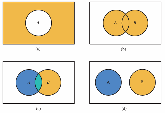
Probability properties (union and intersection)

∀A, 0 ≤P(A) ≤1.
2 If S is the sample space for an experiment, P(S) = 1.
3 P(A∪B)=P(A)+P(B)−P(A∩B) (See Fig.(c)).
4 If A and B are disjoint P(A∩B) = 0 (i.e. A∩B = ∅), P(A∪B) =P(A)+P(B) (See Fig.(d))
5 ∀A, P(A)+P(¯ A) = 1 (See Fig.(a)).

Conditional Probabilities

Let E and F be two events with P(F) > 0. The conditional probability of E given that F has occurred, denoted by P(E|F) (or also PF(E)), is P(E|F) = PF(E) = P(E ∩F) / P(F)
Likewise,P(F|E) = PE(F) = P(F ∩E) / P(E)
From (1) and (2), we get P(E ∩F) = P(E|F)P(F) = P(F|E)P(E)

Independance 3 equivalences

Two events E and F are said to be independent if P(E|F) = P(E ∩F)/ P(F) =P(E) If P(E|F) = P(E), it is also true that P(F|E) = P(F). <=> P(E ∩F) =P(E)P(F) <=> E(XY)=E(X)E(Y)

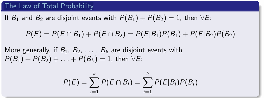
The Law of Total Probability

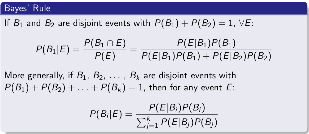
Bayes’ Rule

Random variable

a numerical variable X whose value depends on the outcome of a chance experiment

Discrete

Takes specific, separate values; countable, like whole numbers or events.

Continuous

Takes any value within a range; measurable, like height or time

expected value

E(X) = sum(x * p(X=x)) or integral

Expected values 3 properties

E(aX +bY) = aE(X)+b E(Y)
E(X * Y)=E(X)+E(Y)
E(X⋅Y)=∑​x⋅y⋅P(X=x,Y=y) or E(X⋅Y)=∫[−∞∞]​∫[−∞∞] ​x⋅y⋅fX,Y​(x,y) dxdy

where fX,Y(x,y)f is the joint probability density function of X and Y

Variance

σ^2 X = V(X) = sum( [x −E(X)] ²) . p(X=x) or integral formula

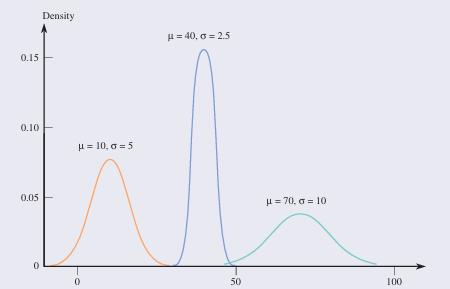
Empirical rule

68–95–99.7 rule

in a normal distribution: approximately 68%, 95%, and 99.7% of the values lie within one, two, and three standard deviations of the mean, respectively

P ( mu - 1*sigma <= X <= mu + 1 sigma) = 68%
P ( mu + 2*sigma <= X <= mu + 2 sigma) = 95%
P( mu + 3*sigma <= X <= mu + 3 sigma) = 99.7%

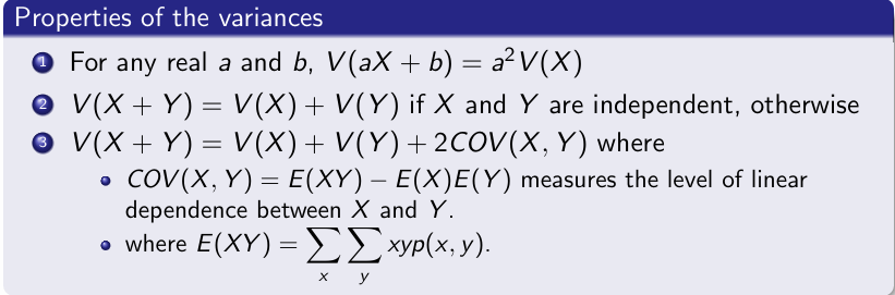
2 Properties of variance + covariance definition

For any real a and b, V(aX +b) = a2V(X)
V(X +Y)=V(X)+V(Y) if X and Y are independent, otherwise
V(X +Y)=V(X)+V(Y)+2COV(X,Y) where COV(X,Y) = E(XY)−E(X)E(Y) measures the level of linear dependence between X and Y.

The correlation coefficient

ρXY ∈ [−1,+1] measures the linear dependence between two random variables X and Y. It is defined as follows:
ρXY = COV(X,Y) / σXσY ∈ [−1,+1]

Note that: The higher ρXY, the more positive the correlation. The smaller ρXY, the more negative the correlation. ρXY = 0 corresponds to an absence of linear dependence.

The higher ρXY, the

more positive the correlation

. The smaller ρXY, the

more negative the correlation

ρXY = 0

corresponds to an absence of linear dependence.

The Bernouilli distribution def + Expected value and variance

is a discrete probability distribution which takes value 1 with success probability p and value 0 with failure probability q = 1 − p. The expected value and variance of a Bernouilli variable X are :
E(X) = p
V(X) = pq

The binomial random variable X def + Expected value and variance

is defined as X = number of successes observed among n trials- seen as a Bernouilli variables. Then, if X is a binomial variable (noted X ≡ B(n,p)), we get: P(X =x)=p(x) =P(x successes among n trials) =( n x) p^x(1−p)^n−x
where (n x) = n! / x!(n−x)! is read as “n choose x” and represents the number of ways of choosing x items from a set of n.
E(X) = np and V(X) = np(1−p)

(n x) formula + def

= n! / x!(n−x)! is read as “n choose x” and represents the number of ways of choosing x items from a set of n.

A probability distribution for a continuous random variable X

is specified by a curve called a density curve. The function that defines this curve is denoted by f(x) and is called the density function. The following are properties of all continuous probability distributions:

1. f(x)≥0 for all x.

2. The total area under f(x)= 1, i.e., ∫[−∞+∞] f(x) dx=1.

The probability that X falls in any particular interval is the area under the density curve and above the interval

A Normal (or Gaussian) distribution

is bell-shaped and symmetric. It is characterized by a mean μ\muμ and standard deviation σ\sigmaσ.

• μ describes where the corresponding curve is centered, and

• σ describes how much the curve spreads out around that center.

The density function of X∼N(μ,σ) is defined as follows:
f(x)=1/sqrt(σ²2π) ​​exp(− (x−μ)²/ 2σ^2

The standard normal distribution

is the normal distribution with μ=0 and σ=1. It is customary to use the letter Z to represent a variable whose distribution is described by the standard normal curve (also called the Z curve).
We get Z from the following transformation: Z=X−µ / σ ≡ N(0,1)

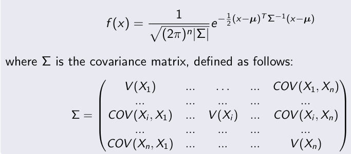
Multivariate Gaussian distribution

Generalization of the one-dimensional (univariate) normal distribution to n dimensions. The density function of X ≡ N(µ,Σ) is defined as follows (where X and µ ∈ Rn)

Central Limit Theorem

Let X1,...,Xn be a sample of n independent and identically distributed (i.i.d) random variables drawn from any distribution (not itself normal) of expected value E(Xi) = µ and variance V(Xi) = σ^2.

If n is large, the sample average ¯ X = X1+...+Xn / n is approximately normally distributed of mean E(¯ X) = µ¯ X = µ
and variance V(¯ X) = σ^2 /n (thus, σ¯ X = σ /sqrt(n)
The Central Limit Theorem can safely be applied if n ≥ 30.

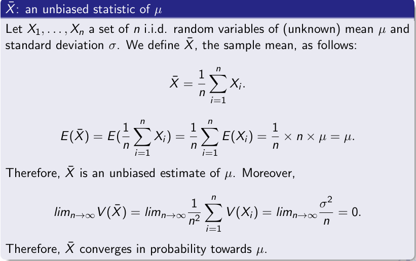
unbiased statistic

A statistic whose mean value is equal to the value of the population characteristic being estimated is said to be an … . More formally, a statistic ˆ θ is an … estimate of the population characteristic θ iff: E(ˆ θ) = θ

Convergence in probability

An unbiased estimate ˆ θ of θ converges in probability iff: limn→∞V(ˆ θ) = 0

X barre: an unbiased statistic of µ

Maximum Likelihood Estimation

Let x1,x2,..., xn be a random set of n i.i.d. observations, each coming from an unknown density function fθ(xi) where θ is a parameter (e.g. p for the binomial distribution, µ and σ for the normal distribution, etc.). The likelihood Lθ of the set corresponds to the joint density function fθ(x1, ..., xn): Lθ = fθ(x1,...,xn) = f (x1|θ) × f (x2|θ) × ··· × f (xn|θ) = product of the f (xi|θ)

Estimate thanks to Maximum likelihood estimation

To find an estimate ˆ θ as close to θ as possible, one solves: ∂Lθ / ∂θ = ∂fθ(x1,...,xn) /∂θ = 0

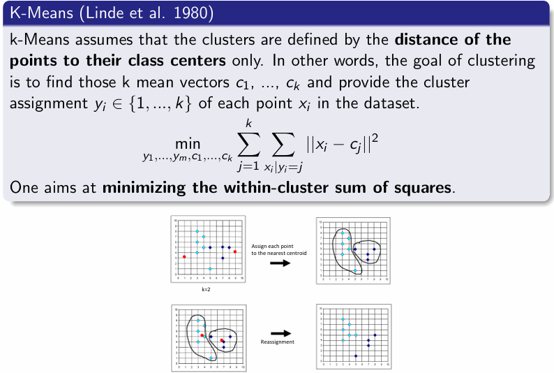
K means

assumes that the clusters are defined by the distance of the points to their class centers only. In other words, the goal of clustering is to find those k mean vectors c1, ..., ck and provide the cluster assignment yi ∈ {1,...,k} of each point xi in the dataset. k min y1,...,ym,c1,...,ck sum sum ||xi − cj||^2 knowing that j=1xi|yi=j One aims at minimizing the within-cluster sum of squares.

determinant

For n ≥ 2, the determinant of an n ×n matrix A = [aij] is the sum of n terms of the form ±a1j ×det(A1j), with plus and minus signs alternating, where Aij is the submatrix formed by deleting the ith row and jth column of A.

inversible matrix

Let A be a n×n square matrix. If det(A)= 0 then A is … (or non singular).
If det(A) = 0, then A is not … (or singular matrix).

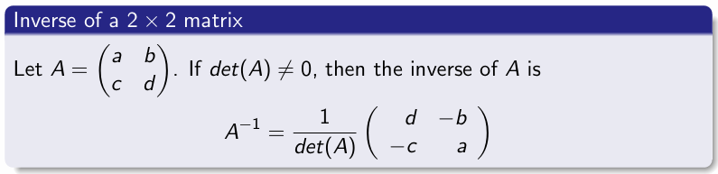
2 × 2 matrix inverse

1/ det(A) (d - b -c a )

The Invertible Matrix Theorem

Let A be a square n ×n matrix. Then, the following statements are equivalent:
1 A is an invertible matrix.
2 A is row equivalent to the n ×n identity matrix.
3 A has n pivot positions.
4 The columns of A form a linear independent set.
5 The columns of A span Rn (canonical basis of Rn).
6 A^T is an invertible matrix.

Trace

sum of diagonal tr(A) = a11 +... +ann

Trace properties

tr(A +B) = tr(A)+tr(B) (only holds for square matrices).
tr(cA) = c ×tr(A) (only holds for square matrices)
tr(A) = tr(AT) (only holds for square matrices).
Key properties used in many proofs: if a ∈ R, tr(a) = a
tr(AB) = tr(BA) (also true with A and B resp. m ×n and n×m matrices)
tr(A^TB) = tr(AB^T) = tr(B^TA) = tr(BA^T) (also true with A and B defined as m ×n and n×m matrices).
tr(ABC) = tr(CAB) = tr(BCA) (also true with A, B and C resp. m ×n and n×m and m×m matrices)

Eigenvectors and Eigenvalues

The eigenvectors of a square matrix A are the non-zero vectors that, after being multiplied by A, remain parallel to the original vector. For each eigenvector x, the corresponding eigenvalue λ is the factor by which the eigenvector is scaled when multiplied by the matrix. More formally, x is an eigenvector of A if there is a scalar λ such that Ax = λx.

Eigenvalues

The eigenvalues of A are the solutions λ to the following characteristic equation: det(A − λI) = 0
det(A) = Product( λi)

2×2 Matrix eigenvalue

if A is a 2×2 matrix, then the characteristic equation takes the form of λ^2 −tr(A)λ+det(A) = 0.
Therefore, λ = tr(A)± sqrt( tr(A)^2 − 4det(A)) / 2

Convex optimization problem

problem minimize f0(x) subject to fi(x) = 0, i = 1,...,m where the objective and constraint functions are convex.

Convex

A function f is convex if f (ax +(1−a)y) ≤ af(x)+(1−a)f(y)
∀x,y ∈ Rn, and ∀a ∈ [0,1].

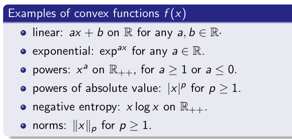
Examples of convex functions

linear, exp, power, power of abs, negative entropy, norms p>=1

differentiable

A function f : Rn → R is … if its derivative exists at all x ∈ Rn. Then the gradient of f at x is the vector whose components are the partial derivatives of f at x: ∇f(x1,..., xn) =( ∂f / ∂x1 ,··· , ∂f / ∂xn )^ T

Suppose f is differentiable, then f is convex if

∀x,y: f (y) ≥ f(x)+∇f(x)T(y −x)
if ∇f (x) = 0 then it means that x is the global minimizer of f .

Second order condition:

A twice differentiable function f is convex iff its Hessian ∇2f(x) is PSD.

Positive semi-definite (PSD)

A matrix M ∈ Rn×n is positive semi-definite (PSD), denoted M ⪰ 0, if all its eigenvalues are ≥ 0. The complexity of checking M ⪰ 0 is O(n^3). It can be done by hand for very small matrices, but when M gets large, it becomes costly even for a computer.

2×2 Hessian matrix convexity

The determinant det(H) ≥ 0.
So, λ1 and λ2 have the same sign or one = 0 (since det(H) = λ1 ×λ2)

The trace tr(H) > 0. So, λ1 and λ2 are both positive or one is positive and the other = 0 (since tr(H) = λ1 + λ2).

IF Hessian Positive definite (PD)

then the function is strongly convex

The method of Lagrange multipliers

provides a strategy for finding the extrema of a function f subject to equality constraints h, by changing the original constrained problem into an unconstrained optimization one
minw f(w) subject to hi(w) = 0,i = 1..n
To solve the previous problem, let us construct the Lagrangian:
Λ(w,λ) = f(w)+ sum(λi * hi(w) )
where parameters λi are called Lagrange Multipliers (or Dual Variables, that have to be found)

Lagrangian for R²

To simplify, let’s assume that Λ(x,y,λ) = f (x,y) + λh(x,y). Finding the optimal solution (x∗,y∗) requires to compute the following partial derivatives set to 0.
∂Λ /∂(x,y,λ) =0
This leads to set ▽f +λ.▽h=0 (1)
h(x,y) = 0 (2)
Equation (1) means that the two gradients of f and h must be collinear at the optimal point (x∗,y∗).
Equation (2) means that the solution must also satisfy the constraint.

For lagrangian multipliers : ▽f +λ.▽h=0 means ?

that the two gradients of f and h must be collinear at the optimal point (x∗,y∗).

For lagrangian multipliers : h(x,y) = 0 means ?

means that the solution must also satisfy the constraint

Non regularized Least Squares Problem

Goal+ math

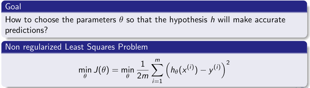
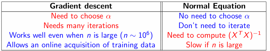
How to minimize J(θ)?

Batch Gradient Descent
Stochastic Gradient Descent
Mini-Batch Gradient Descent
Closed-form solution

Let us assume that J(θ) is differentiable: Start with some initialization of θ (e.g. ⃗ θ = 0 or some randomly chosen vector.)
Update θ’s values so that to reduce J(θ) (by computing partial derivatives of J(θ) w.r.t. θ).
Repeat the process till convergence to the minimum of J(θ).
θi := θi −α ∂ J(θ) / ∂θi

if J(θ) is differentiable then

it decreases fastest in the direction of the negative gradient of J(θ)

alpha in gradient descent

is the learning rate which controls how large a step you take in the direction of the steepest descent.

Large versus small learning rate α

For some specific examples, J(θ) may increase. This may occur in such following situations where α is large (“zigzag” effect)

Stochasting and mini batch struggle to get to the minimum how to resolve this issue ?

In most implementations, the learning rate is held constant. However, if you want to converge to “a minimum” you can slowly decrease α over time, such that at iteration i we get: αi = C1 / i +C2 , which means you’re guaranteed to converge “somewhere”

Mini-batch gradient descent

is a variation of the gradient descent algorithm that (randomly) splits the training dataset into small batches that are used to calculate model error and update model coefficients.
… descent seeks to find a balance between the robustness of stochastic gradient descent and the efficiency of batch gradient descent

Closed-form Solution definition

A mathematical problem is said to have a closed-form solution if, and only if, at least one solution of that problem can be expressed analytically in terms of a finite number of certain ”well-known” functions

closed-form solution for linear regression

Therefore, solving
∇θJ(θ) set =⃗0 boils down to solving:
X^T X θ−X^T y = 0
X^T X θ = X^T y (Normal Equation)
we get: θ = (X^T X )^-1 X^T y (closed-form solution)

Context where (X^T X)^-1 is non-invertible

Redundant features (linearly dependent, i.e. rank(XTX) < n)
Example: x1: size in feet2 and x2: size in m2. We know that x1 = 3.28x2.
= >Possible solution: perform a PCA (see next chapter).

Too many features

=> Solution: delete some features before (using feature selection algorithms).

→These limitations explain why gradient descent approaches are sometimes preferred

polynomial reg

y =θ0+θ1x +θ2x2 +...+θnxn. Note that the regression function is still linear in terms of the unknown parameters θ0, θ1, θ2 etc.
Therefore, we can address the problem by using a standard multiple regression model where x1 = x, x2 = x2, x3 = x3, etc. are distinct variables

Error term

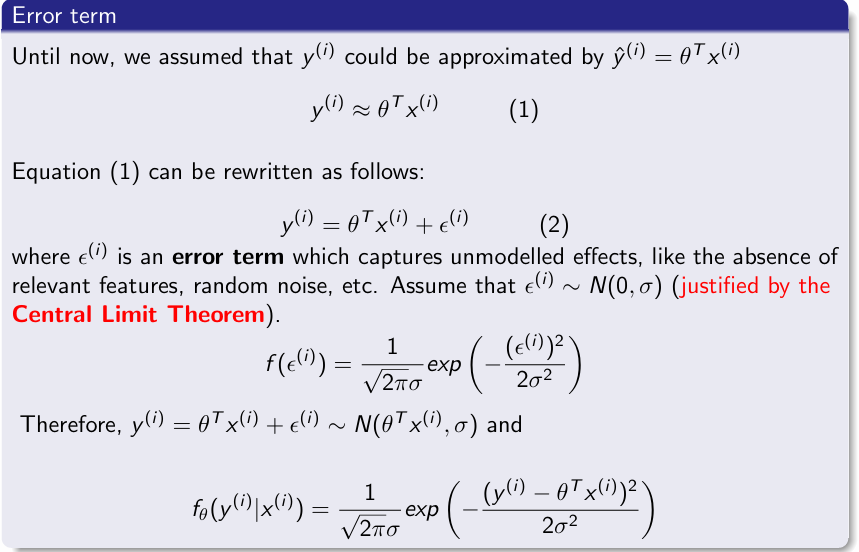
The ordinary least square algorithm

is just maximum likelihood assuming i.i.d gaussian errors on the data.

Methods to prevent overfitting in Linear Regression

Regularized versions of Linear Regression

1 Ridge Regression (using the ℓ2-norm).

2 LASSO (using the ℓ1 norm).

Ridge regression

is based on the ℓ2 norm and penalizes the size of the regression coefficients. The optimization problem is the following one:
(X^T X + λI)^-1 X^T y

Least Absolute Shrinkage and Selection Operator (LASSO)

makes use of the ℓ1 norm to constrain the algorithm to remove irrelevant features. It bounds the sum of the absolute values of the coefficients. The optimization problem is defined as follows:
t turns out that increasing the least square penalty will cause more and more of the parameters to be driven to zero

LASSO stands for ?

Least Absolute Shrinkage and Selection Operator

SVR: Support Vector Machine Regression

Support Vector Machine Regression (SVR) predicts continuous values using support vectors, epsilon margins, and kernel functions for flexible, robust modeling.

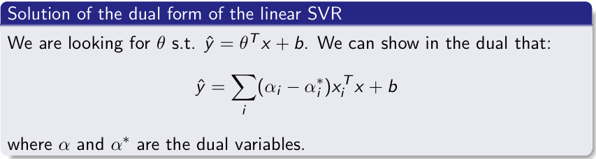
Solution of linear SVR

y = (αi −αi* )xi^T x + b
where α and α∗ are the dual variables.

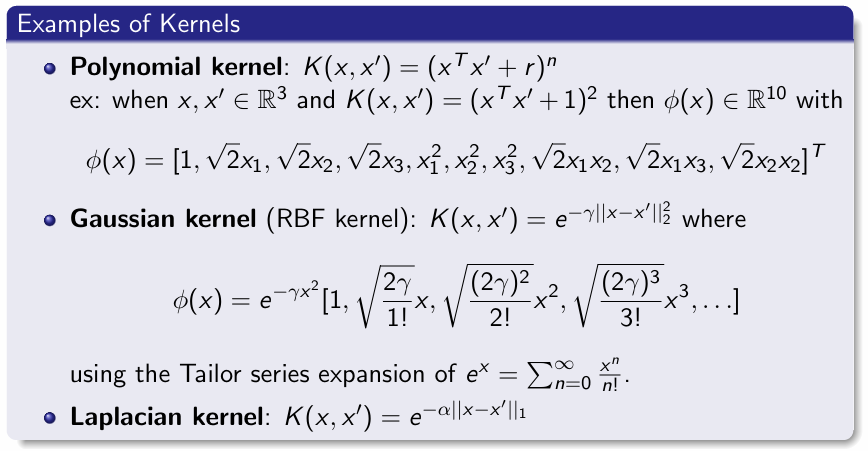
Kernel trick

The kernel trick avoids the explicit mapping by using a kernel function K : X ×X →R satisfying that K(x,x′) = ϕ(x)Tϕ(x′).

Examples of kernel

Polynomial kernel

Gaussian kernel

Laplacian kernel

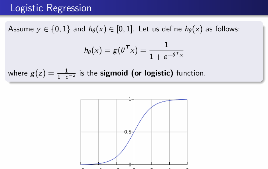
Logistic regression

Logistic regression models binary outcomes using a logistic function, estimating probabilities based on independent variables for classification tasks.

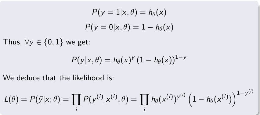
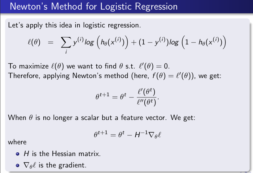
Likelihood of logistic regression

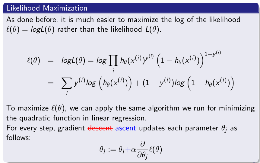
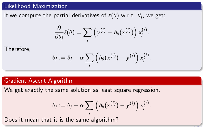
log Likelihood Maximization

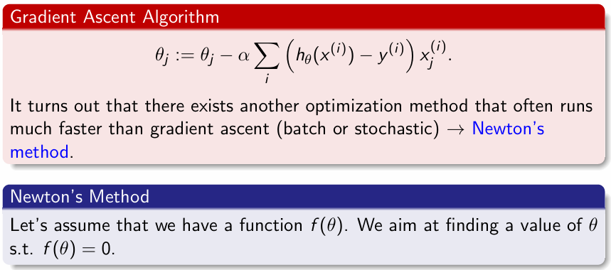
Gradient ascent algorithm

Therefore, behind the logistic regression there is ?

x is classified 1 if it is above the line θTx = 0 and 0 otherwise. …, there is a linear classification model θTx = 0 which splits the space into two parts.

Newton’s method

By the definition of the gradients, f ′(θ) at a given iteration is equal to the vertical length f (θ) divided by the horizontal length ∆. Therefore, at iteration 1, we get: f ′(θ0) = f (θ0)/ ∆ and∆= f(θ0) /f ′(θ0)

More generally, one iteration of Newton’s method updates θt as follows: θt+1 = θt − f(θt) /f ′(θt)

Newton method for logistic regression

PROS For a reasonable number of features and training examples, Newton’s method converges more quickly than gradient ascent in far fewer iterations.

At each iteration, we need to invert the n×n Hessian matrix (where n is the number of features). Therefore, if n is very large, it is expensive.

If some conditions are not met, it is not guaranteed to converge. E.g. (i) some starting points may enter an infinite cycle, or (ii) when we start iterating from a point where the derivative is zero

Newton method doesn’t converge in which conditions ?

(i) some starting points may enter an infinite cycle, or
(ii) when we start iterating from a point where the derivative is zero

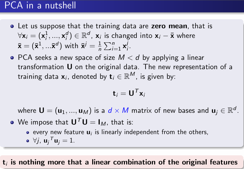
PCA

Find a lower-dimensional feature space while preserving the underlying stucture (i.e. the variance) of the original data (If the dimensionality reduction leads to a 2D-feature space, PCA allows data visualization).

Look for principal components and use them to perform a change of basis of the data

Thus PCA performs a feature extraction by generating linearly uncorrelated features that might bring meaningful information.

PCA stands for

Principal component analysis

Goal of PCA

is to linearly project the data xi ∈ Rd onto a space having dimensionality M < d such that close points in that new M-space mean similar examples in the original d-space.

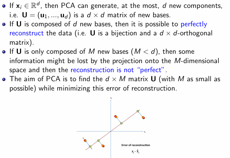
Reconstruction after PCA

If xi ∈ Rd, then PCA can generate, at the most, d new components, i.e. U = (u1,...,ud) is a d × d matrix of new bases. If U is composed of d new bases, then it is possible to perfectly reconstruct the data (i.e. U is a bijection and a d × d-orthogonal matrix). If U is only composed of M new bases (M < d), then some information might be lost by the projection onto the M-dimensional space and then the reconstruction is not “perfect”. The aim of PCA is to find the d ×M matrix U (with M as small as possible) while minimizing this error of reconstruction.