All Diagrams

Economics HL 2023 Course

1.1 PPC Curve

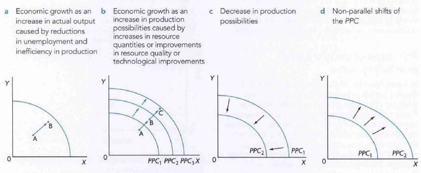
1.1 PPC Curve

PPC: A visual representation of all possible combinations of two types of goods that can be produced with given factors of production

• Assumed that all resources must be fully employed and used efficiently

• Assumed that the state of technology remains the same

• However, output is always below frontier in real world due to unemployment of resources (higher unemployment= further away from point)

• Scarcity, choice and opportunity cost are always taken into account

  • Curve shows maximum resources that can be utilised

  • PPC displays the law of increasing opportunity cost (the more produced of one thing, the more of the other thing that needs to be forgone)

  • Further down the curve, one thing is benefitted more than the other

  • Shape of PPC displays opportunity cost of producing goods and services

  • Various combinations, e.g. gives up laptops for phones

  • An economy's actual output or quantity of output produced is always inside the PPC because real world economies will always have unemployment of resources and inefficiency

1.2 Circular Flow of Income Model (closed)

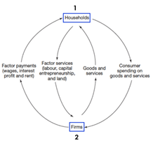
Displays that in any given time period, the value of the output produced in an economy is equal to the total income generated in producing that output, which is equal to the expenditures made to purchase that output

• then just explain each flowy thing

1.3 Circular Flow of Income (open with leakages & injections)

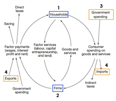
A more realistic model in RW

• Savings and Investment: investment is spending by firms for the production of capital good. savings=leakage, however if invested into e.g. banking of finance firms obtain funds that flow back into expenditure and act as injections

• Taxes and G Spending: household pay through taxes=leakage because income is not spent on goods and services. But government spends tax funds (education/health…) therefore=injection

• Imports and exports: imports purchased by domestic buyers= leakage because they represent household spending that leaks out payments to other countries, exports produced domestically and purchased by foreigners= injection because they are spending by foreigners who buy goods and services produced by the domestic firms

  HOWEVER, in the real world leakages and injections are unlikely to be equal which has consequences to the size of circular flow.

  • if injections>leakages the size of the flow increases

  • if injections<leakages = decreases

  • OFTEN matched but not equal

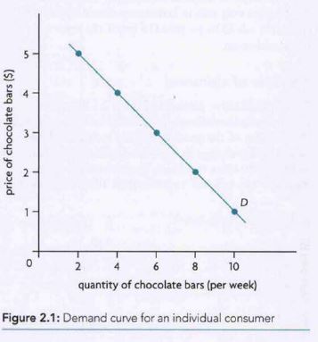
2.1 Market Demand Curve

the summation of all the individual demand curves based on overall market demand. (is a display of how quantity demand relates in variation in prices) *draw a negative linear function

• shift in curve= change in demand

• movement along the curve caused by a change in price (this is the change in quantity demanded)

  o   Expansion: quantity demand increases (fall in price)

  o   Contraction: quantity demand decreases (rise in price)

  o   Shifts Right: demand increases

  o   Shifts Left: demand decreases

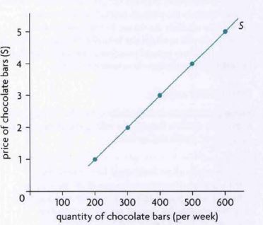
2.1 Market Supply Curve

the summation of all the individual firms’ supply curves based on overall market supply (displays how quantity supplied relates to variation in prices)  *draw a positive linear function

• o   Extension: upward movement
  o   Contraction: downward movement
  o   Shifts Right: increase in supply
  o   Shifts Left: decrease in supply

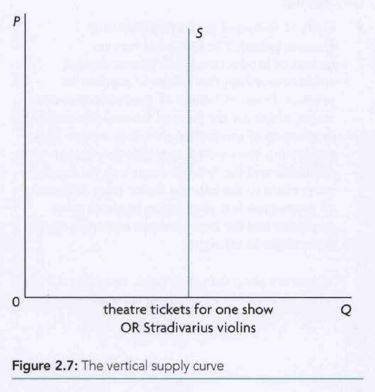
2.2 Vertical Supply Curve

Regardless of price, quantity will be fixed
Example: antiques, quantity of seating in synonym

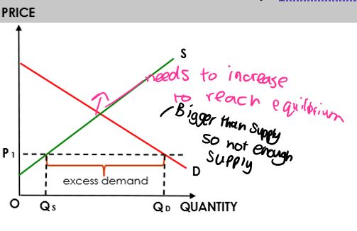
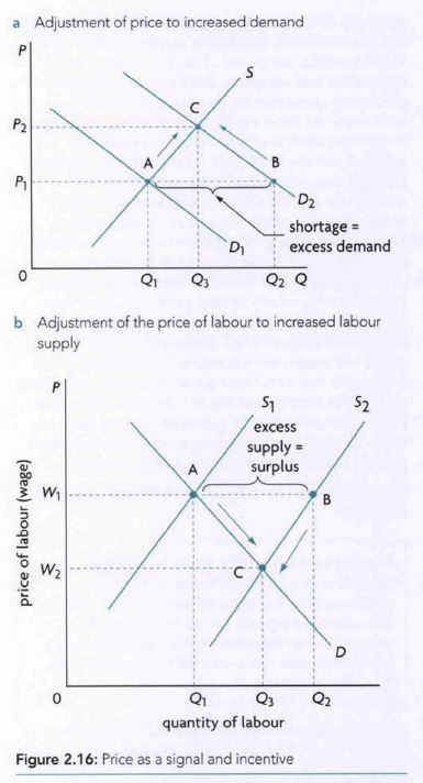
2.3 Demand & Supply Curve

A representation of the amount of a commodity, product or service available

• Excess Demand= demand>supply

• To reach equilibrium again= increase price

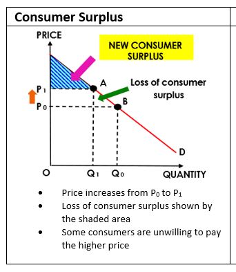
2.4 Consumer Surplus

Consumer Surplus: the price that consumers are willing and able to pay on a good or service vs what they actually pay↑consumer surplus= ↓market price (vice versa)

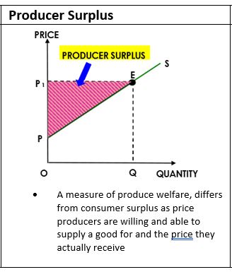
2.5 Producer Surplus

the difference between the price producers are willing and able to supply a good or service for and the price they actually receive↑producer surplus= ↑market price (vice versa)

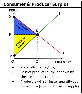
2.6 Consumer & Producer Surplus

a surplus which arises because some consumers are willing to pay more than the given price for all but the last unit they buy

2.7 Price Mechanisms

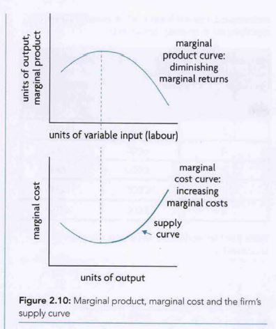
2.8 law of diminishing marginal utility

when marginal product increases, marginal cost decreases vice versa

the firm’s supply curve is a portion of it’s marginal cost curve that shows the price-quantity combinations where the extra cost of producing one more unit of output is equal to the price of that unit

3.1 PED Diagrams

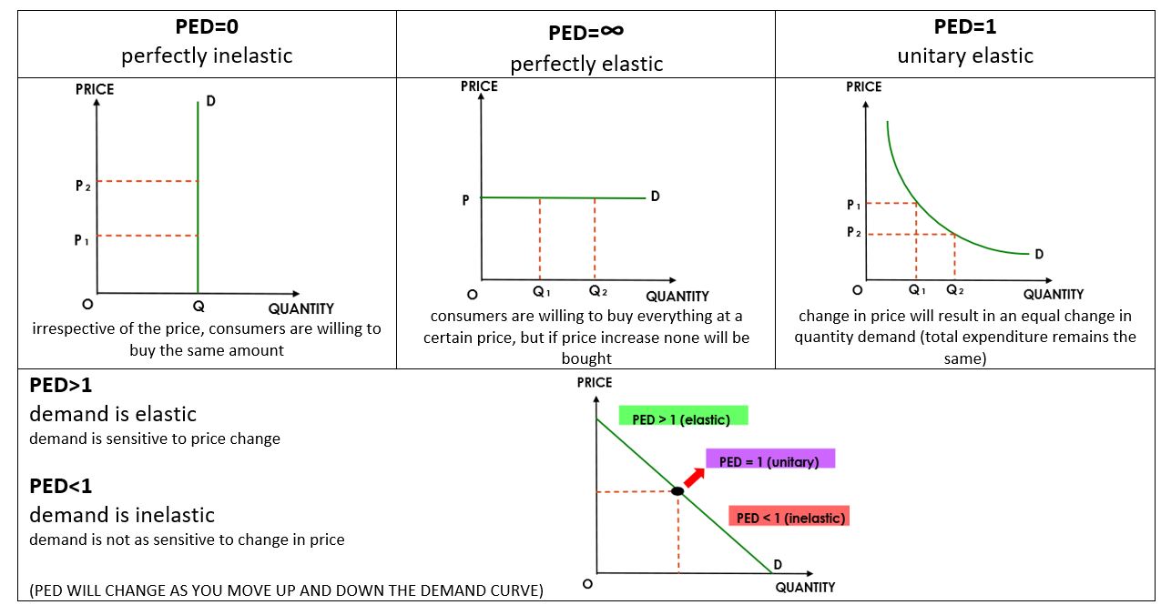
Steepness:

• flatter=more elastic

• steeper= more inelastic

3.2 PED firm and pricing decisions

• businesses take PED in account when considering changes in the price of their product

• to increase total revenue it must deop price if demand is elastic

3.3 PED firm and indirect taxes

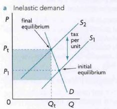
• gov imposes taxes on specific goods

• if gov are interested in increase tax revenues they must consider PED of the goods being taxed

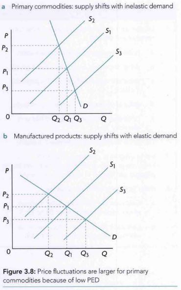
3.4 PED in relation to primary commodities and manufactured products

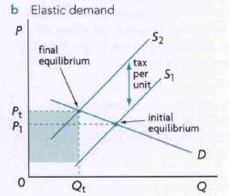
• primary goods (natural resources), manufactured goods are not

• when low PED for primary commodities creates problems for producers and result in flucatuations of commodity prices

• both diagrams show effects on the price and quantity when there is a decrease in supply or increase om supply

3.5 YED

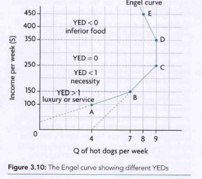
3.6 The Engel Curve

• more accurately illustrates YED then demand curve shifts

• Engel Curves are all points representing the quantities demanded of the goods at various levels of income, when prices and preferences are held constant

3.7 PES

4.1 Price Ceilings (price control)

4.2 Price Floors (price controls)

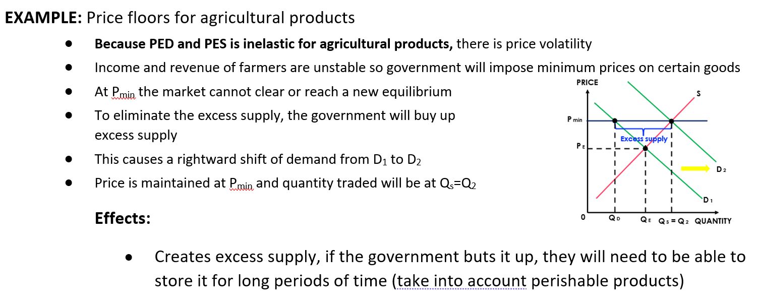
4.3 Market ourcome from indirect tax

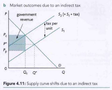
4.4 Specific Tax

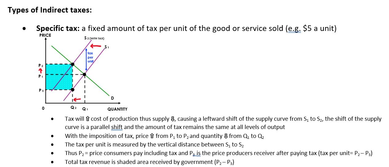
4.5 Ad valorem tax

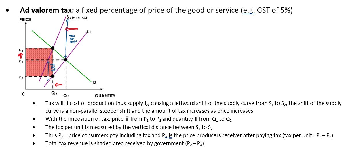
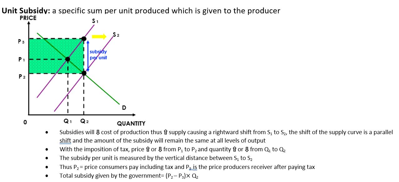
4.6 Unit Subsidy

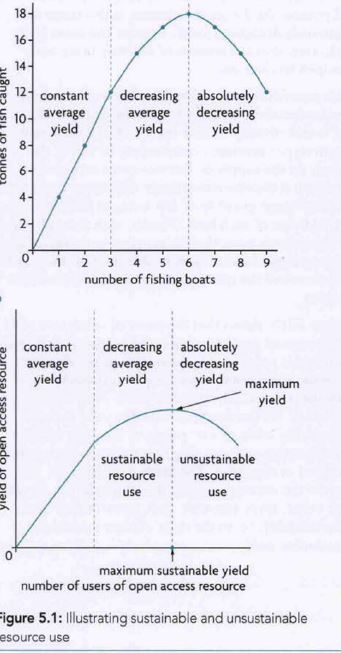
5 The Tragedy of Common Pool Resources:

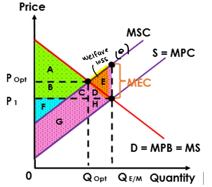
5.2 Negative production externalities

·       Consumer deman curve = MPB = MSB

·       Producer’s supply curve = MPC

·       Socially desired point where MSC=MSB

·       Cost of NPE: MSC=MPC+MEC

·       Welfare loss where MSC>MSB indicates actual output>socially desired output

·       If the firm was more responible and produces less than Q_opt there would be no welfare loss

to fix: indirect taxes

market based policies: carbon taxes, tradable permits

5.3 Negative consumption externalities

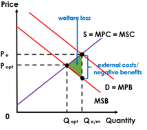
·       Producer supply curve= MPC= MSC

·       Negative externalities caused by traffic congestion= negative benefits (-MEB)

·       Socially desired point where MSC=MSB

Welfare loss where MSC>MSB where there is overallocation of resources

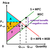
6.1 positive production externalities

·       At Q_e/m  MSB>MSC thus too little is being produced due to under allocation of resources

·       Due to underproduction, there is a loss of external benefits to society which creates welfare loss (AT AREA (C))

·       If firms were to be more responsible and produce more at Q_opt the external benefits would be gained and welfare loss eliminated

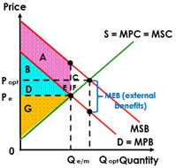
6.2 positive consumption externalities

·       Consumer demand curve= MPB

·       If consumers are aware of external benefits generated D=MPB+MEB=MSB

·       Actual price output: P_e  and Q_e/m

·       Socially desired point is where MSC=MSB

·       Due to underallocation of resources where MSB>MSC there is welfare loss (AREA AT (CF))

If consumers were to be more responsible and demand more at Q_opt the external benefits would be gained and welfare loss eliminated

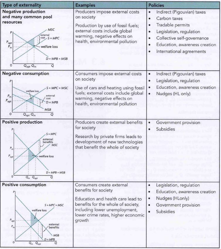
5+6 summary of externalities

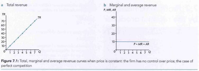
PERFECT COMPETITION: Total Revenue vs Marginal&Average Revenue

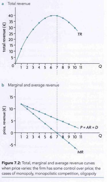
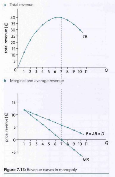
IMPERFECT COMPETITION: Total Revenue vs Marginal&Average Revenue

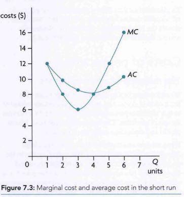
Relationship between Average Cost and Marginal Cost in short run

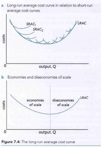
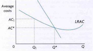
Relationship between Average Cost and Marginal Cost in long run

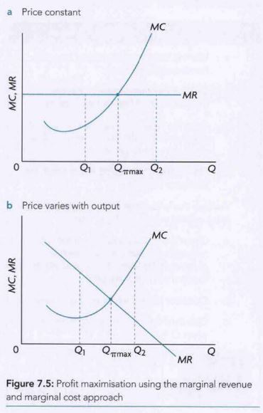
Profit maximisation based on MR and MC Approach

Profit is maximized at q_pm where MC = MR. At output levels less than q_pm, MC is less than MR so expansion of output adds more revenue (MR) than costs (MC). At output levels greater than q_pm, profit is increased by reducing output since the reduction in revenue, MR, is less than the reduction in costs, MC.

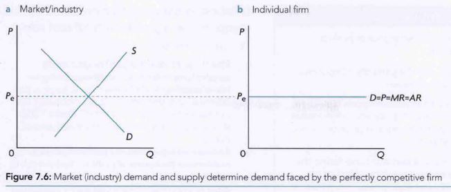
Demand and Supply determine demand from a perfectly competitive firm

PERFECT COMP: Profit maximisation in the short run

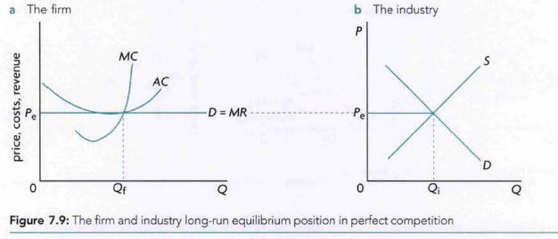
PERFECT COMP: Profit maximisation in the long run

revenue curves in monopoly

natural monopoly

consumer and producer surplus in monopoly compared to perfect competition

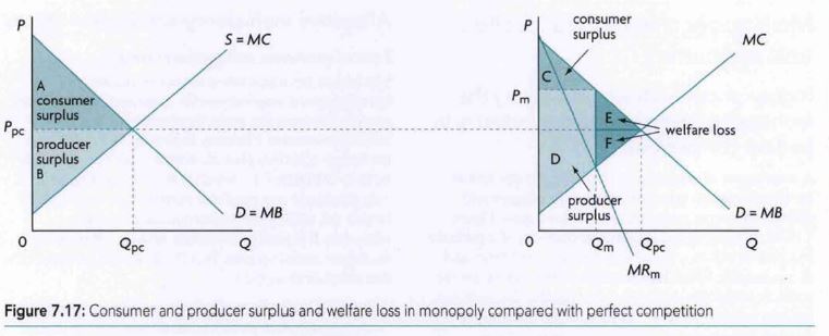
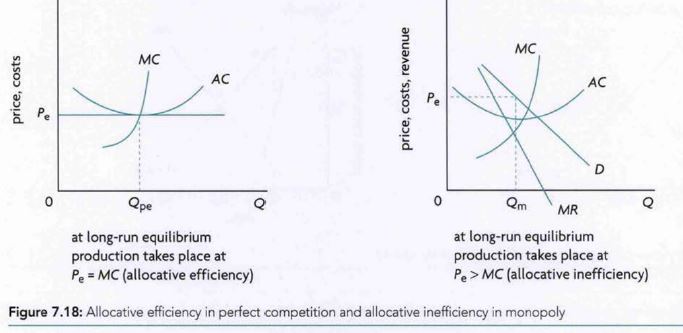
allocative efficiency in perfect competition and allocative inefficiency in monopoly