Week 9: Species Abundance Distribution + The Latitudinal Diversity Gradient (LDG)

Biological structure of a community

the mix of species, including both their number and relative abundance

Species richness

number of species that occur within a community

Relative abundance

percentage each species contributes to the total number of individuals

Rank- abundance plot

graphical way to show relative abundance

Species evenness

equitable distribution of individuals among species

Why are large carnivores/ predators rare?

loss of energy/ inefficient transfer→ differences between trophic levels

a histogram showing the number of individuals per species on the x axis (arithmetic scale) against the number of species in that class on the y axis

• hollow curve pattern

• few common species → many species have a low abundance

• many rare species → few species have a high abundance

• one of ecologies universal laws

Rank-abundance plot (Whittaker plot)

most common = rank 1

least common = rank n (n = number of species)

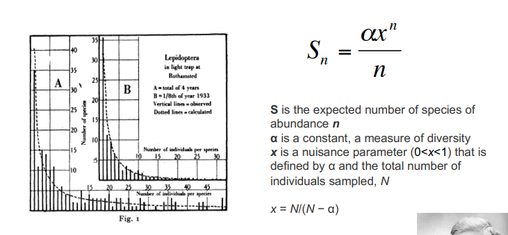
Log Series

Fisher R. A. et al. 1943

• Ronald Fisher → analysed species-abundance

• moths → light traps

• hollow curve pattern can be seen

• uneven distribution of abundance

• larger alpha = more evenly distributed abundance

• N+ alpha on slide not N- alpha

• According to the log-series, singleton species are the modal class

What did Frank Preston argue?

• log-series like distribution is a sampling artefact due to failure to sample the rarest species

• most datasets represent samples rather than complete enumerations

Preston, F.W. (1948) The commonness, and rarity, of species. Ecology, 29, 254–283.

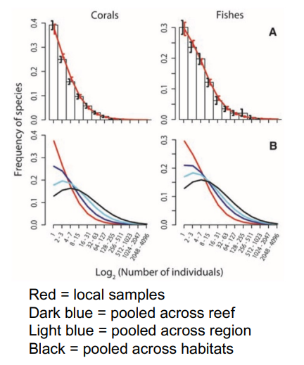
Log normal

• Preston, 1948

• Plotting well sampled communities with the x-axis on a log-scale reveals an intermediate peak

• modal class of intermediate abundance: log-normal

• normally distributed on log scale + sampling enough→ log normal

• octaves

• each class double the number as before

• species consisting of 1 individual less than species consisting of 2-3

• Preston veil line

More recent study backing up log normal distribution

• Conolly et al (2005) Community Structure of Corals and Reef Fishes at Multiple Scales, Science 309: 1363

• increase in sampling → log normal distribution emerges

Variation in shape of SAD in tropical communities vs. temperate

• tropical rain forest trees look log -normal but look at whole rainforest → hollow curve

• tropics → more species, more evenly distributed

• opposite to temperate zones

• tropical forest trees on completely sampled plots log-normal like

• understory plants in Irish conifer plantation log-series like

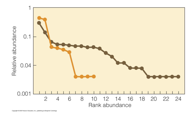
What did Alroy show in a 2015 paper?

Alroy 2015 The shape of terrestrial abundance distributions. Science Advances

• variation in both richness and evenness among communities

• tropical communities (black) have shallower rank abundance plots -> more even distribution of abundance

• temperate communities (grey) dominated by a few species

What did Anne Magurran show in Magurran & Henderson (2003) Nature?

• more than one pattern

• Estuarine fish, Bristol, 21 years

• Discontinuity between persistence and maximum abundance

• Ever present core species: Log-Normal

  • 1 group → always there, high abundance → log modal

• Transient: Log-series

  • other group→ not consistently there → log series

Potential Explanations

• abundance of rare species controlled by random dispersal events

• other group → controlled by availability of resources

Why does detecting abundance matter?

• impacts of human activity on biodiversity

• abundance in disturbed vs. undisturbed

Link between disturbance and SAD

Hill et al. (1995) J. Applied Ecology, 32754-760

• Butterfly species across forest transects in Indonesia

• undisturbed: Log-normal like (solid symbols)

• disturbed: Log-series like (open symbols)

• disturbed → more uneven distribution

Estimating Diversity of Floral Species in the Amazon basin

ter Steege, H. et al. 2013 Hyperdominance in the Amazonian Tree Flora

• Estimates of local tree abundance from 1195 plot samples: sample includes ~5,000 species

• Compared 16 different statistical SAD models: log-series fit best

• Use log-series to predict the unsampled species as well as their abundance

• Estimated 16,000 species across the Amazon basin

• 227 (1.4%) account for half of all individual trees

• The rarest 5800 species have estimated population sizes of <1000→ species may never be discovered

Why is it important to estimate the floral diversity in the Amazon?

important finding as forests are carbon sinks

→ conserve the few 100s of tree species + understand response to environmental change for most of the forest

What processes explain the shape of SADs?

1. Central Limit Theorem

2. Niche apportionment models

3. Neutral theory

Example of population growth being determined by the multiplicative (synergistic) effect of different resources

Elser, J. J., et al. 2007. Global analysis of nitrogen and phosphorus limitation of primary producers in freshwater, marine and terrestrial ecosystems. Ecology Letters

• Addition of both nitrogen and phosphorus results in higher plant productivity than expected based on the effect of each resource in isolation

What is the central limit theorem?

May, R. M. 1975. Patterns of species abundance and diversity

• The multiplicative effect of many independent variables acting on population growth would lead to a ‘lognormal’ SAD

Nekola and Brown 2007 The wealth of species: ecological communities, complex systems and the legacy of Frank Preston

• The abundance of many things in nature, not just species abundance, show lognormal patterns

Niche apportionment models

Tokeshi (1990) Niche apportionment or random assortment: species abundance patterns revisited

• The local abundance of a species depends on the amount of resources available to that species

• Relative abundance thus reflects resource division among species •

• Imagine a resource pool (we might call this ‘niche space’) utilized by a species. A new species invades the community and takes a fraction of these resources, and this process is repeated

• Leads to a ‘hollow curve’ pattern

• Many different ways of theoretically dividing niche space that lead to different shaped SADs

Dominance pre-emption (DP) model

• Each species arrives and takes up a constant proportion of the remaining resources

• K=0.5

  • First ranked 50% of total abundance/biomass

  • Second ranked 50% of remaining 50% = 25%

  • Third ranked = 12.5% of total abundance

• Generates a ‘geometric series’ distribution

• Characterized by a straight line (with slope k) on the rank-abundance diagram

why 50%

→ no theoretical explanation for the fraction of resources species should take

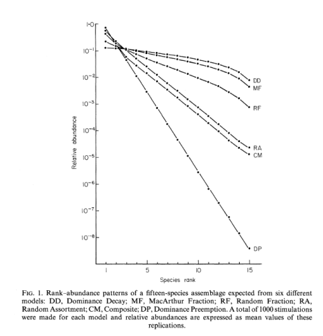
Dominance decay (DD) model

• Dominance decay (DD) is the inverse of DP

• top line of the graph

• It is always the largest niche that is divided

• Results in a more even distribution

• Random assortment (RA) niches are selected at random and split at random

• Intermediate level of evenness

• log-normal like

How did neutral theory begin?

• The unified neutral theory of biodiversity and biogeography

• started as a theory in genetics →most mutations neither deleterious/ selected for

• no positive + negative effect → explanation for huge variation

Rosindell et al 2001 The unified neutral theory of biodiversity and biogeography at age ten.

What did Stephen Hubbell (2001) argue?

too many tree species to be explained by the partitioning of niche space given all plants depend on a few limiting resources (light, water, phosphorus, nitrogen)

How can so many species co-exist? (Stephen Hubbell)

• niche partitioning → are there so many different niches?

• Tree species coexist, not because their niches are different, but because the have equal fitness (ability to grow + reproduce)

• similarity in fitness allows them to co-exist → one species can’t out-compete another because same fitness

How does neutral theory work e.g within a tree community?

• ‘Zero sum game’ i.e. total number of individuals in local community and in the region is fixed. As one individual dies it is replaced by another (of the same or different species)

• All individuals, regardless of species identity, are identical in terms of their ecology and fitness and have equivalent probabilities of death, producing an offspring or dispersing i.e. the model is neutral at the individual level

• These random processes cause ‘ecological drift’, as the abundance of each species randomly fluctuates over time

• Eventually each species will drift to extinction until there is only one species remaining

• Individuals randomly mutate to become new species (speciation), balancing extinction -> dynamic equilibrium

Zero sum game

plot with fixed number of individuals → zero sum game

Shape of abundance distribution: Neutral Theory

• J (size of regional pool)

• v (speciation rate)

• Number of sites (size of local community)

• θ = 2Jv

  • Small ~ geometric series of abundances

  • Medium ~ log-Normal distribution

  • Large ~ flat (even) distribution

• Fits to rain forest data

Comparing neutral and niche models

• Volkov et al. 2003 compared niche (log normal model) and neutral model in predicting the abundance of trees on Barro Colorado island, Panama

• Neutral model (green) fit better than the niche (black) model

• Relative abundance of species due to neutral processes?

• But similar predictions despite fundamentally different assumptions

• Abundance patterns alone insufficient to resolve the processes structuring communities

What should happen if abundance is set by niches?

Ricklefs and Renner (2012)

• if abundance is set by niches then families of trees abundant on one continent should also be abundant on other continents (if we assume they have retained similar niches)

• Continents have been separated for tens of millions of years and so these correlations are not predicted by the random drift in abundance that occurs in the absence of niches (i.e. neutral theory)

Stronger tests of niche and neutral models

Harpole & Tilman (2006), Non-neutral patterns of species abundance in grassland communities

• Neutral + niche models provide a similar fit to the relative abundance of plant species in the Cedar Creek experiment

• Neutral theory predicts that abundance is independent of the niche

• Harpole and Tilman (2006) found a –ve relationship between R* and biomass

• R* = level to which species reduce soil nitrate when grown in monoculture

• Lower R* = Higher competitive ability

Is neutral theory a sufficient explanation for patterns in species abundance?

• probably not

• But the theory highlighted the importance of regional processes (speciation, dispersal) and chance events in structuring communities

• Resulted in stronger interrogation of empirical data and realization that the shape of SADs alone are not sufficient to discriminate between different theories

One hectare of tropical rainforest can contain…

• 400 tree species (Kraft 2008

• 900 plant species (Balslev 1998)

• More than all tree species in Europe

  • ~16,000 tree species in Europe

What is the Latitudinal Diversity Gradient (LDG)

• Most species on Earth live in the tropics

• The number of species found in a given area declines from the tropics to the poles

• This pattern is repeated across many different types of organisms, from plants to birds, and ants to fish

• the first order biodiversity pattern

Historical Observations of LDG

• The much greater biological diversity of the tropics compared to temperate zone was clear to early naturalists, like Darwin, Bates, Humboldt and Wallace

• Bates (1892) wrote of collecting more than 700 species of butterflies within an hour's walk of his home in Para, Brazil (compared to ~60 resident species in the UK)

Papers showing LDG

Economo et al. 2018 → LDG in ants

Davies et al. 2008 → LDG in mammals

Papers showing LDG in aquatic animals

Collen et al. 2014. Global patterns of freshwater species diversity, threat and endemism

• freshwater biodiversity = highest in amazon basin

Tittensor et al. 2010. Global patterns and predictors of marine biodiversity across taxa

• marine organisms → highest diversity = coral triangle

What drives these large scale gradients in biodiversity?

• No comprehensive answers

• Mix of abiotic factors (e.g. energy, heterogeneity, stability, area), chance (e.g. mid-domain effect), historical events (e.g. ice ages) and biotic interactions (e.g. competition)

Why is it hard to find out what causes LDG?

• can’t easily do (manipulative) experiments on large scales

• long to wait for results e.g of evolutionary processes driving these gradients

• just have a single planet → can’t compare with other places

Theory: Energy Availability

• Curvature of the Earth results in greater solar energy at the tropics, driving higher net primary productivity (production of plant biomass) where water is not limiting

• Plant species richness strongly predicted by AET (the quantity of water (mm/yr) removed from a surface by evaporation and transpiration)

• Statistically explains >70% of the variation in richness

• higher input of energy cascades up food chains to support more species at higher trophic levels

Currie, D. J. (1991)

AET

• Actual evapotranspiration

• The quantity of water that is removed from a surface due to the processes of evaporation and transpiration

Correlation between bird species richness and AET

Storch et al 2007

• positive correlation

• energetic limits to species richness

• lots of energy → lots of food

• support a higher density of individuals

More individuals hypothesis (MIH)

• The local density and species richness of birds increases with energy availability across N America and Europe

• With a higher total number of individuals, rarer species are supported at a higher abundance, reducing rates of stochastic extinction

• Higher energy → more individuals → more species

Mönkkönen, Forsman and Bokma, (2006)

Exceptions that prove the rule: Endothermic mammals and ectothermic marine predators

• looking at smaller taxonomic levels → counter example e.g penguin species richness

• can be informative when thinking about the mechanisms driving the patterns

• Ectothermic marine predators show expected LDG, but richness of endothermic birds and mammals peaks at high latitudes

• metabolic asymmetry

Metabolic asymmetry

• at high latitudes species able to maintain a higher body temperature can attain higher swimming speeds making them better able to capture sluggish ectotherm prey, increasing energy availability to endotherms

• if ability of other fish/ prey you are catching declines = zero sum game

• endotherms → can maintain body temp + swimming speed across different water temps

Grady et al 2019 Metabolic asymmetry and the global diversity of marine predators

Exceptions that prove the rule: brittle star species richness

• Shallow water species: strong LDG predicted by temperature gradients. Higher temperatures provide more kinetic energy for prey capture

• Deep water species: uniform temperature. Peak in richness at high latitudes and continental margins where more chemical energy

More individuals hypothesis (MIH): Manu National Park, Peru vs. Hubbard brook, USA

Terborgh et al 1990

• Species richness: 4-5 x higher (160 species at a single point)

• Biomass: ~5 x higher (190kg/km2 )

• Abundance: almost identical! (1920 vs ~2000 individuals km2)

• Perhaps MIH only explains richness gradients at low-intermediate levels of energy availability?

• larger amounts of energy supporting higher biomass → supporting larger birds not higher density of birds

The Mid-Domain Effect

• If species geographic ranges were randomly placed in a bounded domain then richness would be expected to peak at the centre of the domain ‘the pencil box effect’

• Has been suggested as a possible null model for the LDG

• but species have to arise randomly on the surface of the Earth for this to work → speciation more likely in some places than others

Colwell and Lees (200) The mid-domain effect: geometric constraints on the geography of species richness

Why mountain passes are higher in the tropics?

Janzen, 1967

1. the tropics highlands are inhospitable throughout the year for a lowland species (and vice versa) whereas at high latitudes species can cross these barriers during some seasons

2. temperate regions → summer/ winter → habitats moving up and down mountain → don’t get strong geographic isolation

Thermal niches

Tewksbury, Huey & Deutsch 2008 Ecology. Putting the heat on tropical animals

• Stable temperatures enable greater specialisation of species thermal niches

• climate stable in tropics → species evolved to have narrow niches

• temperate species operate over larger temperature ranges

Example of non-random speciation: Lupinus

Hughes and Eastwood (2006) Island radiation on a continental scale: Exceptional rates of plant diversification after uplift of the Andes

• idea that climatic stability → leads to species narrow niches that are stratified at different elevations and that promotes geographical isolation and speciation

• Lupinus, diverse genus of plants. Andean species arose in the last ~1.5 million years

• Given rise to 81 species, amongst the fastest rates of speciation ever inferred.

Theory: More time for evolution in the tropics

• For most of Earth’s history the climate has existed in a greenhouse state, substantially warmer than the present

• Cold environments, now found at high latitudes, have arisen relatively recently

  • last 60 million years = progressive cooling

  • cold environments only ‘recently’ originated → over the last 40-50 million years

• Less time for species to accumulate there?

• Latitude correlated with multiple factors – energy and time. Challenge of only having a single planet and not being able to perform experiments

• But we can test the effect of time using phylogenetic data

‘Tropical niche conservatism hypothesis’

Wiens and Donogue 2004 Historical biogeography, ecology and species richness

• Species inherit their niche from their ancestor

• tropics older → ancestors of clades occurred in tropics

• It takes time for species to adapt and spread into new climates

• colonsing new latitudes hard → evolve new traits / evolutionary innovation - takes time

• e.g. herbaceous growth, deciduous leaves, and narrow water-conducting cells are adaptations to freezing tolerance in plants.

Evidence supporting tropical niche conservatism hypothesis

Economo et al 2018 Macroecology and macroevolution of the latitudinal diversity gradient in ants

• Phylogenetic tree of ~15000 ant species and subspecies

• Ants arose in the tropics >80mya and only spread out of the tropics <40mya

• Species have accumulated at similar rates – no evidence for differences in rates of speciation or extinction

• ant richness increasing at similar rate in extratropical regions compared to tropics but starting later

LDG in the fossil record

Mannion, P (2020) A deep-time perspective on the latitudinal diversity gradient

• The shape and strength of the LDG has varied over geological time e.g. relatively flat LDG for dinosaurs during Cretaceous

• Modern LDG developed over last ~50 million years

• Strong diversity peak in the tropics during ice-house periods and flattening during greenhouse periods?

• but patchy fossil record, sampling bias

Inverse latitudinal gradient in speciation rates for marine fishes

Rabosky et al. 2018

• Speciation rates not highest in tropics for fish → highest at high latitudes

Potential hypothesis

• Rates of speciation in fish fastest a high latitudes where species richness is lowest

• Perhaps tropical communities have reached a ‘carrying capacity’ and ecological niches are full, while the diversity of polar regions is still increasing to fill empty ecological niches

Which 3 fundamental processes control the number of species in a region?

1. Immigration

2. Speciation

3. Extinction

Diversification = Speciation - Extinction

The LDG must be driven by some combination of:

1. Differences in the rates of any, or all, of these processes

2. Differences in the time available for speciation (or immigration)

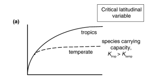
3. Differences in carrying capacity regulating these processes

Differences in carrying capacity

• Negative feedback of standing diversity on diversification and or immigration. e.g. as diversity increases rates of speciation slow down or rates of extinction increase

• The tropics can support more species at equilibrium

• Equilibrium model.

• Mittlebach et al 2007

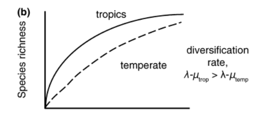
Differences in rates

• Faster rates of speciation, and/or slower rates of extinction and/or faster immigration into the tropics

• Non-equilibrium/historical model

• Mittlebach et al 2007

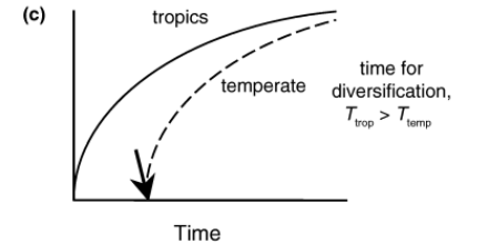
Differences in time

• Tropical climates are older, providing more time for speciation

• Non-equilibrium/historical model

• Mittlebach et al 2007