Unit 6 - Random Variables

probability model

describes the possible outcomes of a chance process and the likelihood that those outcomes will occur

^define sample space (all possible outcomes) and probability for each outcome

random variable

a variable whose value is a numerical outcome of a chance process

*finding probability of event, where possible outcomes are #s _{^{(ex: probability for # of heads when flip a coin) (quantitative variable!)}}

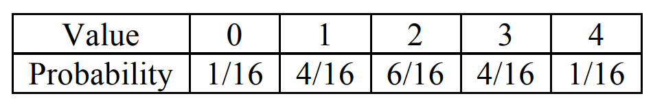
probability distribution

gives a random variable’s possible values and their probabilities

*density curve; histogram, probability vs. random variable X (label x-axis by defining the random variable), analyze w/ SOCS _{^{(compare shape, centers, variance) (can say symmetric for shape) (symmetric means the mean is located at the center b/c it’s the balance point of the distribution)}}

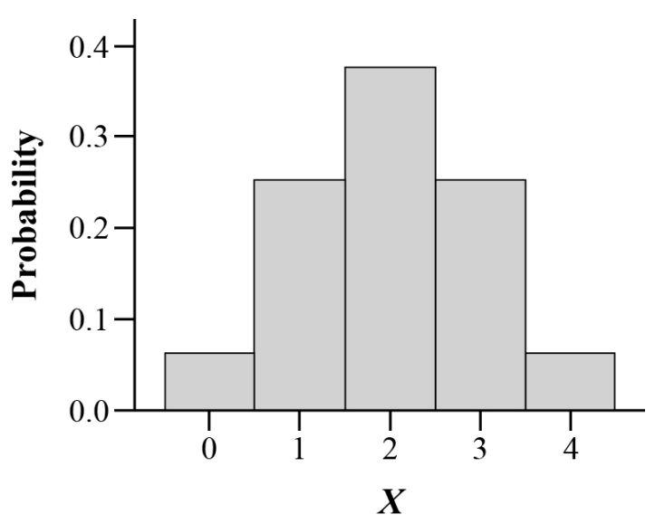
discrete random variable

can list all possible outcomes (value) for a random variable and assign each a probability

*use histogram

Value (numerical outcome): X₁, X₂, X₃

Probability: P₁, P₂, P₃

!!!

interpret P (Probability) → say ‘many many’ and ‘about [P]’

calculator -> use [stat] calc 1-Var Stats → x̄ is mean, σx is SD for discrete random variable

draw normal curve _{^{(always draw for normality!)}} -> draw curve, label N(μ, σ) and axis, draw tick for mean and tick for # in Q, shade appropriate area

if Z = 2X + 3Y → mean: multiply scalars to the means of X and Y then add. SD: multiply scalar to SD first then square. to find σ_Z, must take sqr root of the sum

μ_Z is 2*μ_X + 3*μ_Y

σ_Z² is (2*σ_X)² + (3*σ_Y)² IF X & Y ARE INDEPENDENT (can’t find SD if X & Y aren’t independent) (use this squared eqn if multiple random variables to define a random variable!!) (ex: if only Z = 2X + 3, would just do σ_Z = 2σ_X (Z defined by only one random variable X) (no +3 b/c spread not affected by adding/subtracting))

expected value of X _{^{(a discrete random variable)}}

the mean/avg _{^{(measure of center)}} of the possible outcomes, with each outcome weighted by its probability 

^for each outcome, do value * probability, then sum all of them

μ_X = E(X) = X₁P₁ + X₂P₂ + X₃P₃ + … 

_{^{“incr/decr by about [mean], on avg” / “the mean of [variable] is [mean]. This is the avg [measure of variable] of many, many randomly selected [variable]”}}

SD of X _{^{(a discrete random variable)}}

for each outcome, do value-mean squared times probability, sum for all outcomes, then square root

=√(∑(x_i-μ_X)² * P_i)

_{^{“[event] will typically differ from the mean [mean] by abt [SD] units”}}

continuous random variable

takes on all values in an interval of #s (no gaps) _{^{(find probability of an interval of #s)}} 

^infinitely many possible values, can’t list all     ^use density curve

^for every indiv outcome, P is 0

median lifetime

value m such that P(X ≤ m) = 0.5

^find m using [2nd] [vars] invNorm
_{^{*1/2 success, 1/2 fail}}

!!!

discrete

• #s

• each has probability btwn 0 and 1, sum of all probabilities =1

• fixed set of all possible outcomes/values with gaps in between

• histogram

continuous

• interval of #s

• indiv outcomes have a P of 0 since you're finding probability of intervals

• infinitely many possible outcomes

• density curve

continuous random variable → on calc, use [2nd] [vars]. normalcdf to find probability w/ upper and/or lower bound, invNorm to find value given probability/area under the curve

Transforming random variables

• add/subtract ‘a’ to each observation → changes measures of center/location by a; measures of spread and shape don’t change

• multiply/divide ‘b’ to each observation → changes measures of center/location by b, changes measures of spread by |b|; shape doesn’t change

• Linear transformation, where Y and X are random variables: Y = a + bX

  • Y and X have the same probability distribution

  • μ_Y = a + bμ_X

  • σ_Y = |b|σ_X

  • _{^{compare variance → variance is SD squared, so variance of Y is b² times larger than variance of X}}

• If T = X + Y

  • μ_T = μ_X + μ_{Y ^{(mean of a sum is always the sum of the means)}}

  • σ_T² = σ_X² + σ_Y² (X and Y must be independent random variables!!) ^{_{(variance of the sum is not equal to the sum of the variances, b/c we can't assume that X and Y are independent)}}

• if D = X - Y

  • μ_D = μ_X - μ_Y

  • σ_D² = σ_X² + σ_Y² (X and Y must be independent random variables!!)

_{^{measures of center and location (mean, median, quartiles, percentiles) // measures of spread (range, IQR, SD)}}

independent random variables

when knowing [any event involving X alone] has occurred tells us nothing abt the occurrence of [any event involving Y alone] _{^{(and vice versa)}} 

binomial random variable & setting

perform several independent trials of the same chance process and record the # of times that a particular outcome occurs, where X is the count of successes

CONDITIONS (always check!): 

Binary (success or failure, 2 diff possibilities) 

Independent (trial’s results tell us nothing abt the result of any other trial) _{^{(sampling w/o replacement is not independent, exception is if sample is far less than 10% of the population of interest)}} 

Number (fixed # of trials of a chance process) 

Success (same probability of success on each trial) 

binomial distribution

the probability distribution of X, with n trials and p probability of success on any 1 trial

^possible values of X are whole numbers btwn 0 and n

^binomial distribution shape → more symmetric, approx. normal
*check LCC & 10% condition to approximate binomial distrib w/ normal distrib

^same probability w/ different arrangement (ex: HHFF vs. FFHH)

binomial coefficient 

the number of different ways in which k successes can be arranged among n trials 

→ [math] prob nCr to find coefficient, left put # of trials and right put # of successes
_{^{ex: k=2, n=4: HHFF, HFHF, HFFH, FFHH, FHHF, FHFH (coefficient = 6)}}

finding mean, SD, and probabilities of binomial variables

• μ_X = np 

• σ_X = √(np(1-p))

• binompdf (find exactly k successes)

  • P(X=k)

• binomcdf (find up to k successes)

  • P(X≤k)

• P(X<k) = P(X≤k) - P(X=k)

• P(X>k) = 1 - P(X≤k)

• P(X≥k) = 1 - P(X≤k) + P(X=k) = P(X≥k) = 1 - P(X≤(k-1))

_{^{^n aka x-value is # of trials, p is probability for each success // [2nd] [vars] then up arrow to find binompdf and binomcdf}}

geometric random variable & setting

perform independent trials of a chance process until a success occurs, count the # of trials Y it takes to get the first success _{^{(until first success)}}

^check BINS (but for N, # of trials is not fixed)

_{^{probability p for each success must be the same}}

geometric distribution

probability distribution of geometric random variable Y

*possible values of Y are 1, 2, 3, …

^geometric distribution shape → always right skewed, most common # is 1

finding mean, SD, and probabilities of geometric variables

• μ_Y = 1/p

• σ_Y = √(1-p) over p

• geometpdf (exactly n trials to get first success)

  • P(Y=n)

  • P(Y=n) = (1-p)^n-1p

• geometcdf (takes up to n trials to get first success)

  • P(Y≤n)

• P(Y<n) = P(Y≤n) - P(Y=n)

• P(Y>n) = 1 - P(Y≤n)

• P(Y≥n) = 1 - P(Y≤n) + P(Y=n) = P(Y≥n) = 1 - P(Y≤ (n-1))

_{^{^n aka x-value is # of trials, p is probability of success // [2nd] [vars] then up arrow to find geometrpdf and geometrcdf}}

!!! when taking an SRS of size n from a population of size N, we can use a binomial distribution to model the count of successes in the sample as long as n ≤ 1/10*N (10% condition)
^can infer and use mean and SD formula
^if large population, then SRS w/o replacement is ok and can bypass ‘independent’ in BINS _{^{(^why use 10% for binomial)}} (10% if sample w/o replacement (establish independence))

incr n trials, looks more like normal curve

‘no more than’ is less than or equal to (≤)

how many [] do you expect... -> expected value, mean, do np (binomial) or 1/p (geometric)

_{^{is it legit or not -> if # is suspiciously too high, find probability that X is greater than or equal to that number → P(X≥n) = 1 - P(X≤n) + P(X=n)}}

Large Counts Condition

use normal approximation for a binomial distribution when n is so large such that np ≥ 10 AND n(1-p) ≥ 10 _{^{(the expected # of successes and failures are both at least 10!)}}

^can infer normality and use normal curve

!!! do normal curve for normality

var means variance, variance = SD²

interpret mean/SD: use context, use ‘many many’

• random variable

  • mean: perform many many of chance process, you would expect [random variable] of about [mean], on average.

  • SD: perform many many of chance process, the [random variable] would typically vary around the mean [mean] by about [SD].

• binomial

  • mean: when performing many many trials of n [chance process], the expected number of [desired outcome] is about [mean], on average.

  • SD: when performing many many trials of n [chance process], the # of [desired outcome] varies from the mean [mean] by about [SD].

• geometric

  • mean: if probability of success is [p], when perform independent trials of [chance process] many many times, then expect [mean] trials until get first success

  • SD: when perform independent trials of [chance process] many many times, the typical first [success] will vary by [SD] units from the mean [mean].