gaussian discriminant analysis

univariate gaussian discriminant analysis

Setup (per class k)

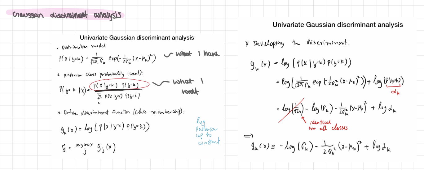
• Assume the feature x inside class k is Gaussian:

P(x∣y=k) = N (x;μ_k​,σ_k²).

Prior of class k: π_k=P(y=k)

What we want for prediction. - posterior class

• P(y=k∣x) By Bayes:

P(y=k∣x) ∝ P(x∣y=k)π_k​

For choosing the class, the denominator cancels—so just compare the scores

score_k​(x)= P(x∣y=k) π_k​

Log-discriminant (same thing, easier math)

g_k​(x) =logP (x∣y=k)+logπ_k​

Plug the Gaussian in and drop the constant −1/2 log⁡(2π) (it’s identical for all classes):

g_k​(x) = − log ⁡σ_k − (x − μ_k )² / 2 σk²_m + log ⁡π _k  

Predict:

ŷ = =argkmax​ g_k​(x)

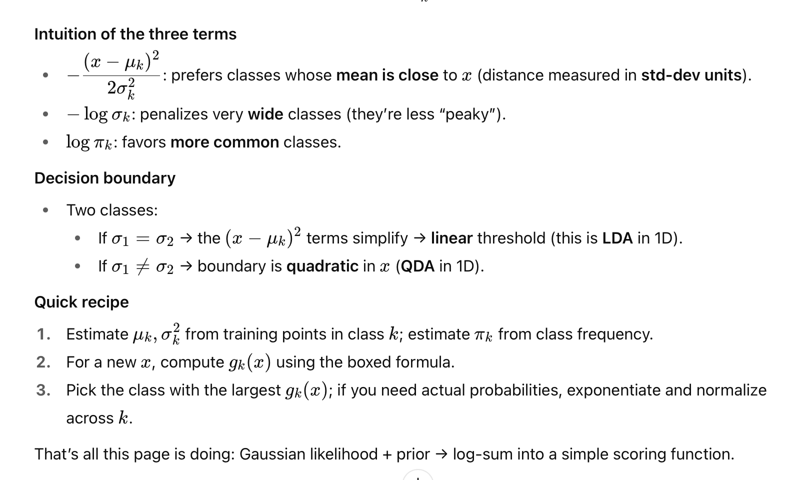
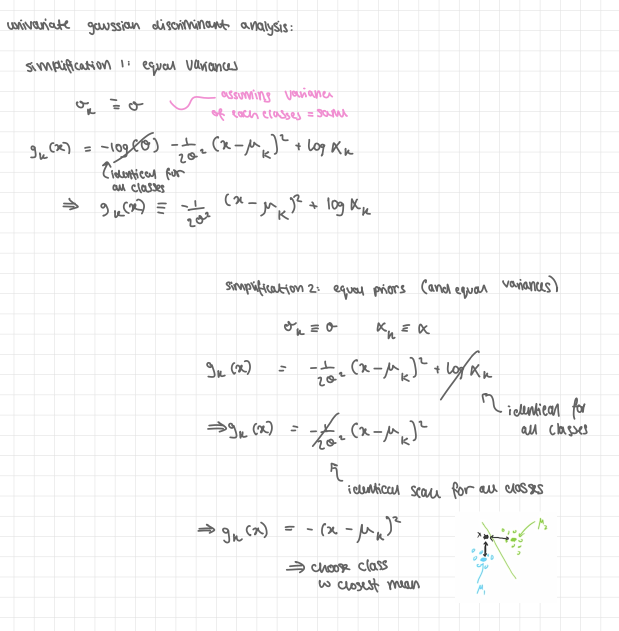
simplifications

GDA collapses to super simple rules under common assumptions

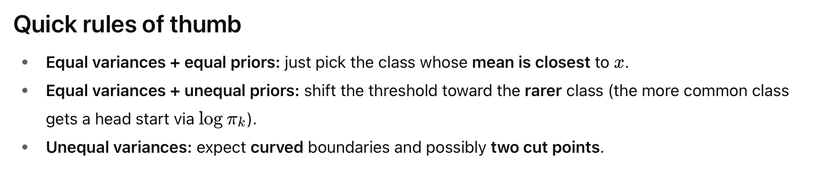
Simplification 1: Equal variances (σ_k=σ for all k)

The −log⁡σ_k term is the same for every class, so it doesn’t affect which is largest

→ g_k(x) = - 1/2σ² (x- μ_k )² + logπ_k

Simplification 2: Equal priors as well (π_k same for all k)

Now log⁡π_k is also common and drops out:

→ - (x- μ_k )² → choose class w closest mean

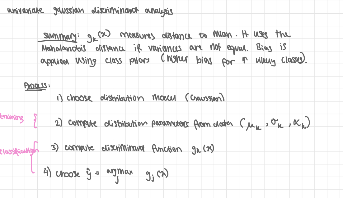
univariate gaussian discriminant analysis summary

g_k(x) measures distance to mean. it uses the Mahalanobis distance if variances Arne’t equal. Bias is applied using class priors (higher bias for more likely classes)

process:

1) choose distribution model (Gaussian)

2) compute distribution parameters from data (σ_k, μ_k , π_k )

3) compute discriminant function g_k(x)

4) choose ŷ = argmax j g_j(x)

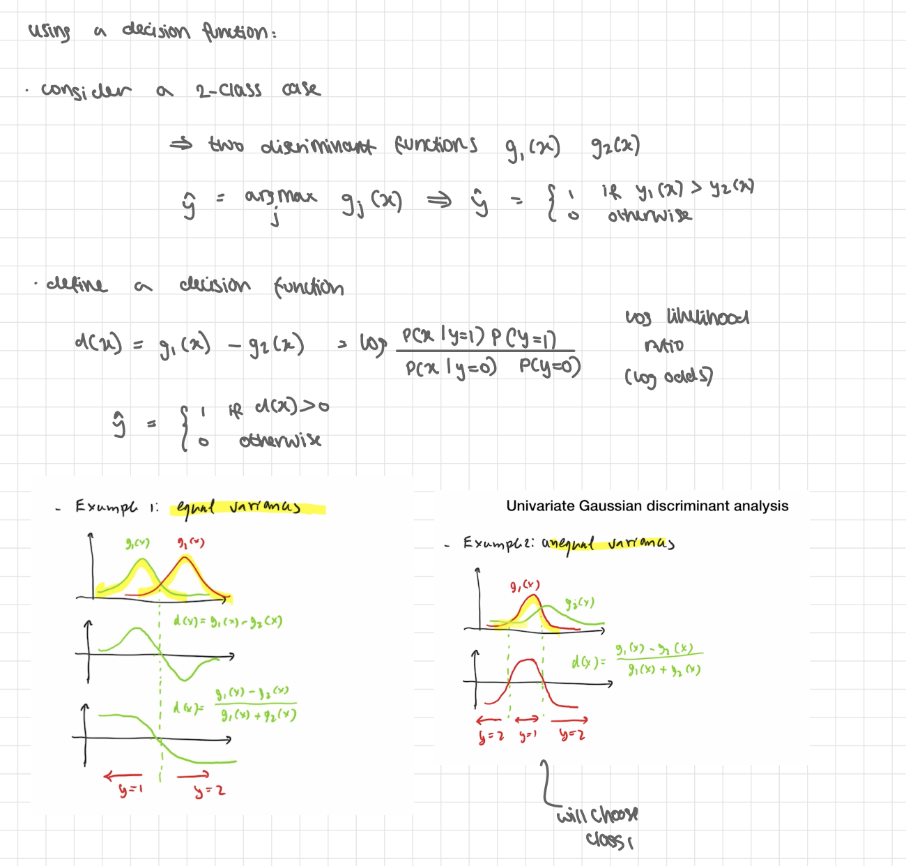
using a decision function

consider a 2-class case

→ 2 discriminant functions g ₁(x) g₂(x)

ŷ = argmax j g_j(x) → ŷ = 1 if y₁(x) > y₂(x) , 0 otherwise

define a decision function

d(x) = g₁(x) - g₂(x) = log (P(x | y=1)P(y=1) / P(x|y=0)P(y=0) ) log odds

ŷ = 1 if d(x) >0, 0 otherwise

multivariate gaussian discriminant analysis

{ (x⁽ⁱ⁾, y⁽ⁱ⁾)}

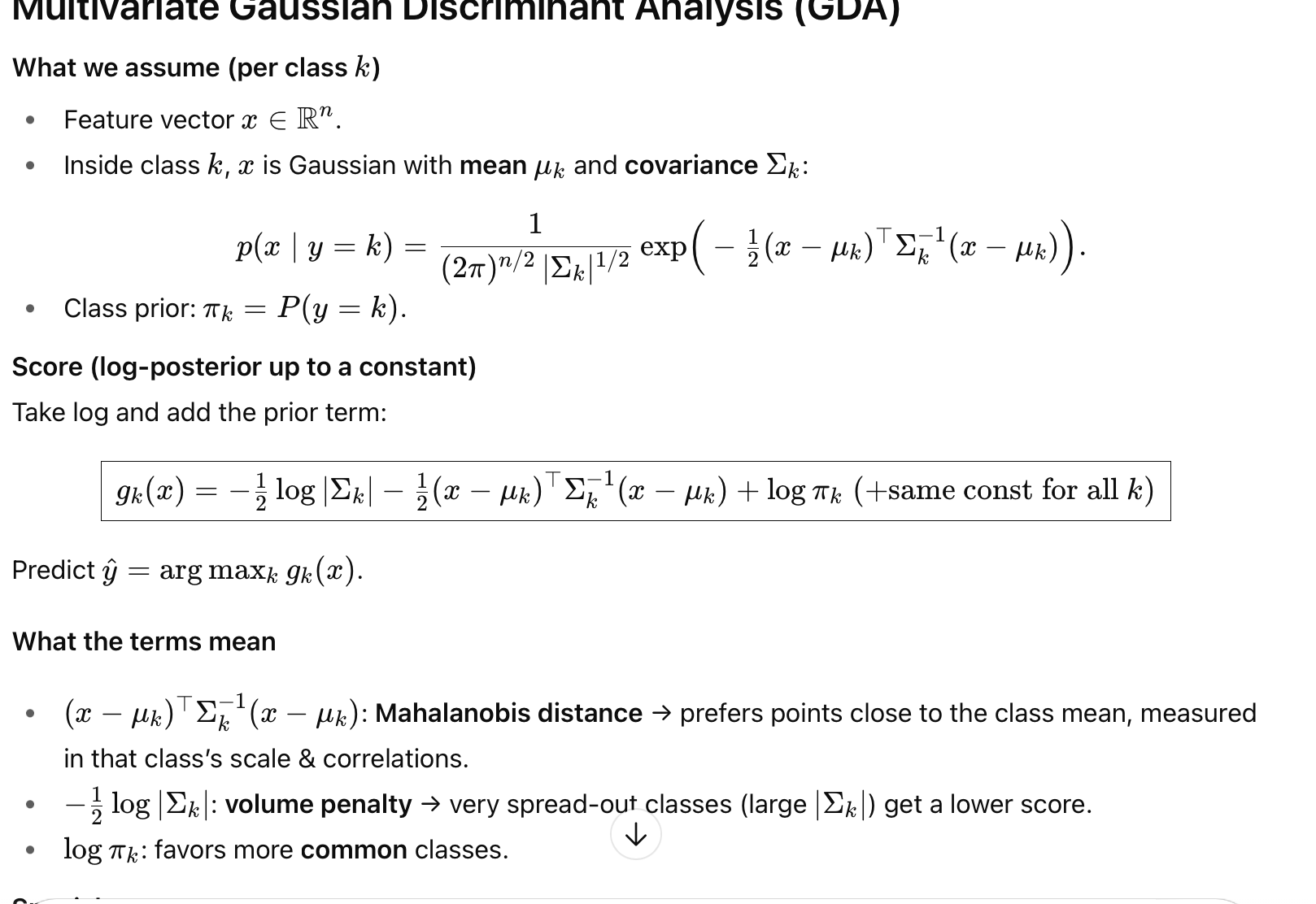
What we assume (per class k)

Feature vector x ∈ R ⁿ

Inside class k, x is Gaussian with mean μ _k and covariance Σ_k :

• (check pic)

Class prior: π _k = P ( y = k )

log-posterior up to a constant:

Take log and add the prior term:

g_k( x ) = −1/2 ​ log∣Σ_k​∣ − 1/2 (x−μ_k)^⊤ Σ_k ⁻¹ ​ (x−μ_k)+logπ_k ​ (+same const for all k)

then predict the label with the biggest g_k(x)

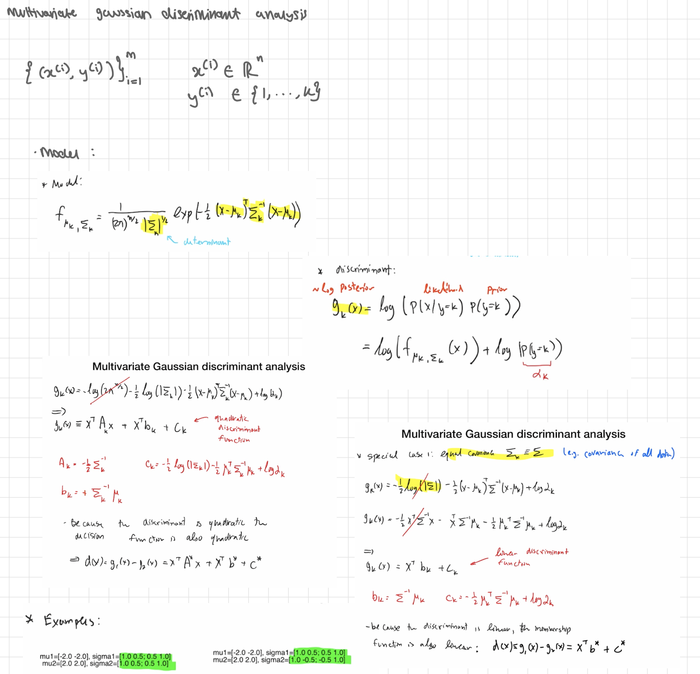
cases

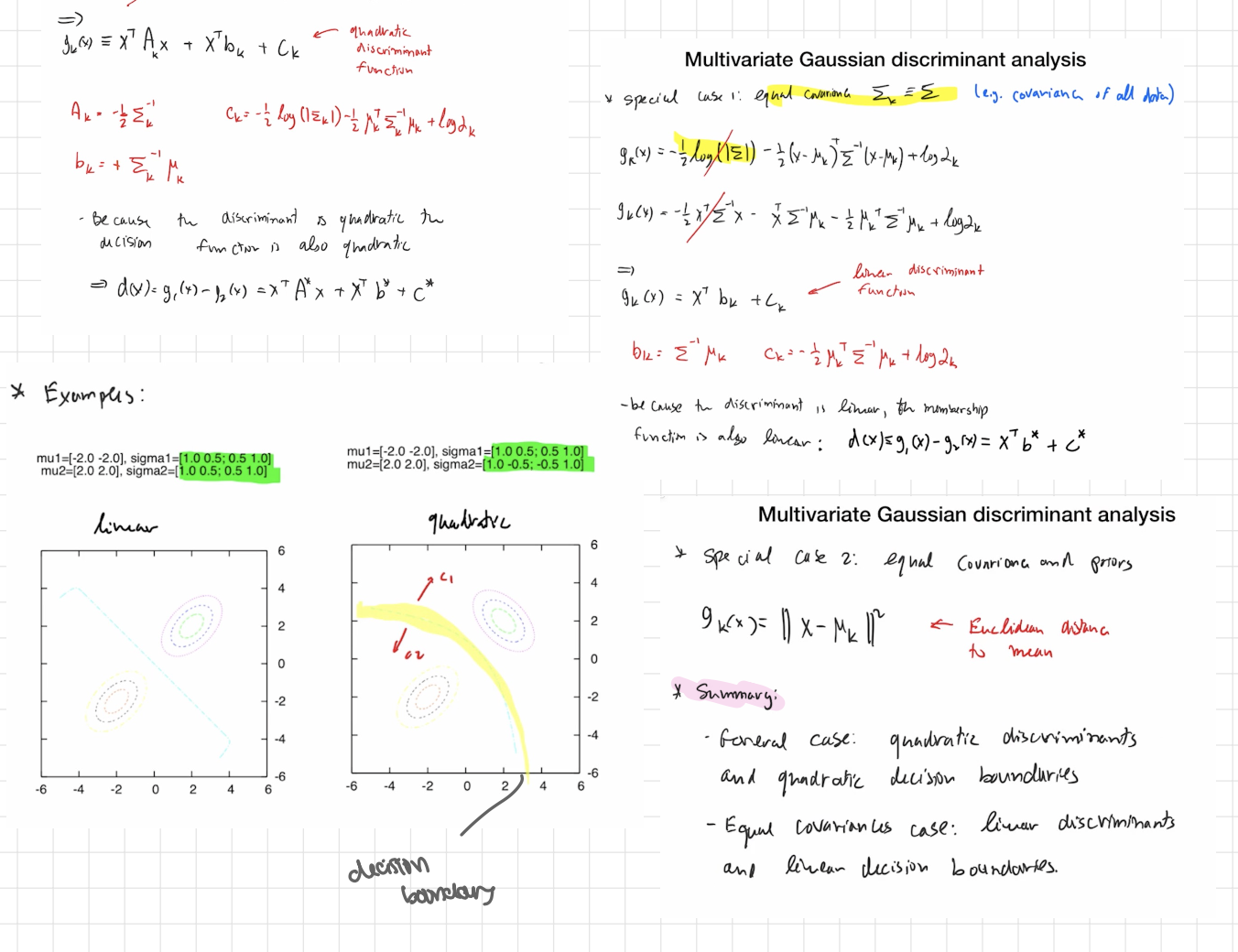
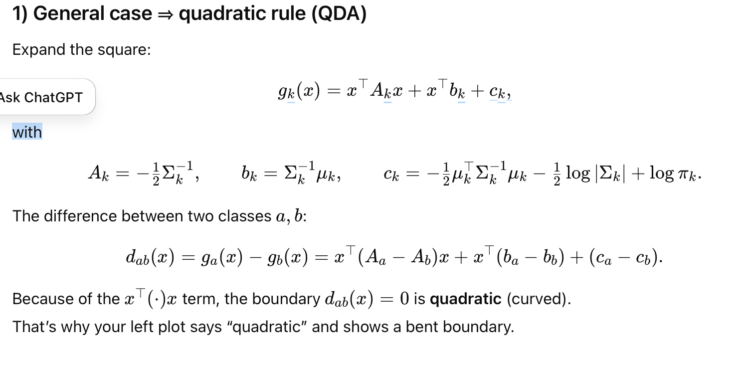
General case ⇒ quadratic rule (QDA)

Expand the square:

• g_k​(x) =x^⊤A_k​x + x^⊤b_k​​+c_k​

with (see pics)

The difference between two classes a,b:

d_ab​(x)=g_a​(x)−g_b​(x)= x^⊤A*x+x^⊤b+ c*

Because of the x^⊤(⋅)x term, the boundary d_ab​(x)=0 is quadratic (curved).
That’s why your left plot says “quadratic” and shows a bent boundary.

Special case: equal covariances (Σ_k=Σ for all k) ⇒ linear rule (LDA)

The quadratic terms cancel (A_a=A_b), so

• g_k(x)=x^⊤b_k+c_k,

• b_k=Σ⁻¹μ_k,    c_k​=−1/2 ​μ_k^⊤​Σ⁻¹μ_k+logπ_k

Decision boundary between two classes is a hyperplane (a straight line in 2D)

special case 2: equal covariances and equal priors

Then log⁡π_k is the same for all k and drops out.

• gk_​(x)= || x - μ_k || ²   ← euclidean distance to mean

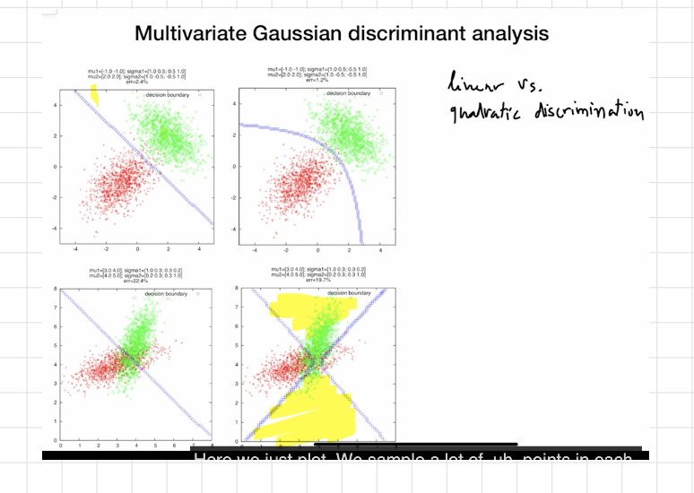
How to read your plots

• Linear panel: same Σ for both classes → straight boundary.

• Quadratic panel: different Σ_k (e.g., one class more elongated/tilted) → boundary bends; you can even get multiple disjoint regions in 1D.

TL;DR

• Different covariances → QDA → Quadratic boundaries.

• Same covariance → LDA → Linear boundaries.

• Same covariance + priors → pick the closest mean (Euclidean if spherical).

js image

estimating distribution parameters

maximum likelihood (MLE)

What we’re estimating (per class k)

• Prior π_k=P(y=k) → how common the class is

• Mean μ_k → average feature vector in class k

• Covariance Σ_k→ spread/shape of features in class k

Pick parameters θ that make the observed data most probable:

θ^=argθmax​ L(θ), L(θ)=P(all data∣θ).

With the standard i.i.d. assumption (examples are independent and identically distributed):

L(θ)= ⁱ⁼¹∏_m​ P(x⁽ⁱ⁾,y⁽ⁱ⁾∣θ).

Independence ⇒ product over i.
Identical ⇒ each term uses the same parameters θ

We almost always maximize the log-likelihood (sums are easier than products):

ℓ(θ) = logL(θ) =ⁱ⁼¹∑_m​ logP (x⁽ⁱ⁾,y⁽ⁱ⁾ | θ).

estimating distribution parameters

Goal:

Estimate the Gaussian parameters for each class k: the mean μ_k and variance σ_k² (and the prior π_k by Maximum Likelihood (MLE).