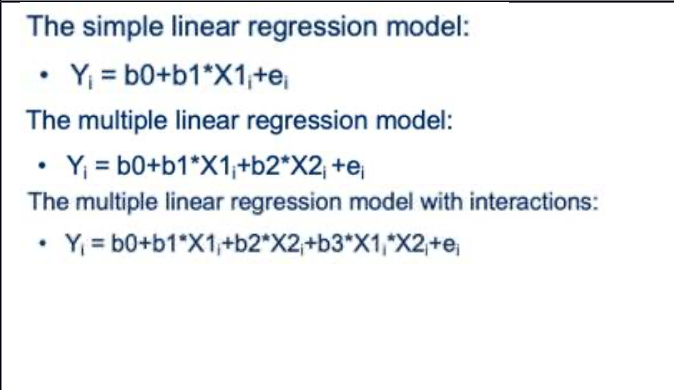
Linear regression 1

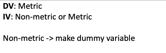
1. Measurement scale

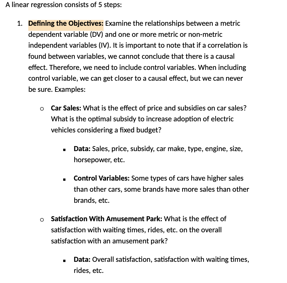
1. Defining the Objectives:

2. Designing the Linear Regression:

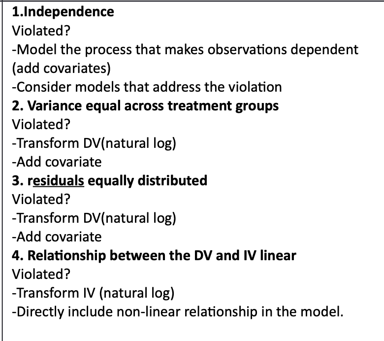
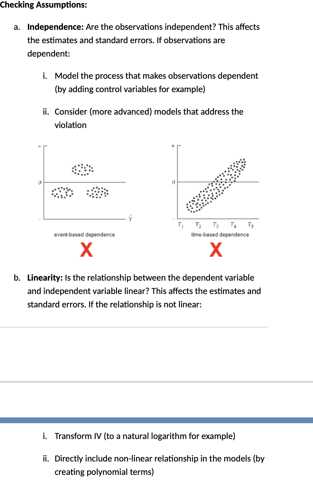
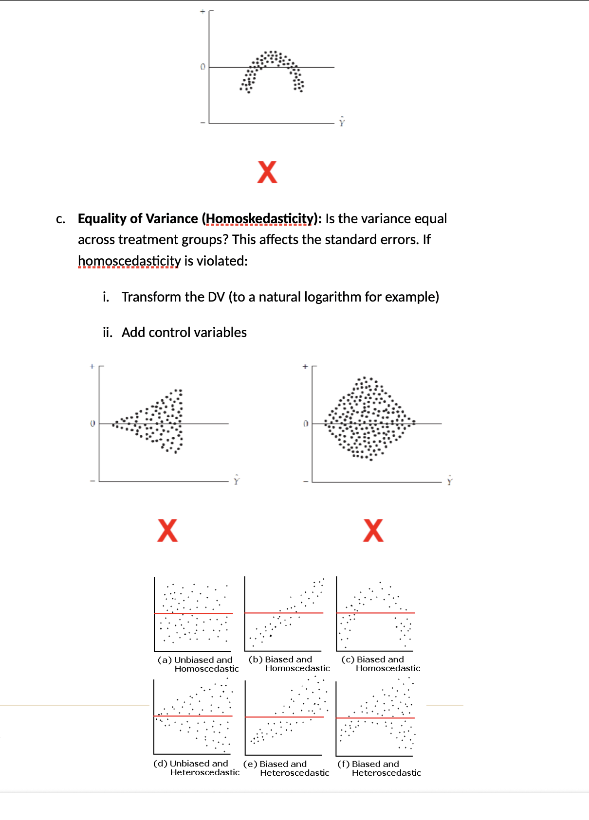
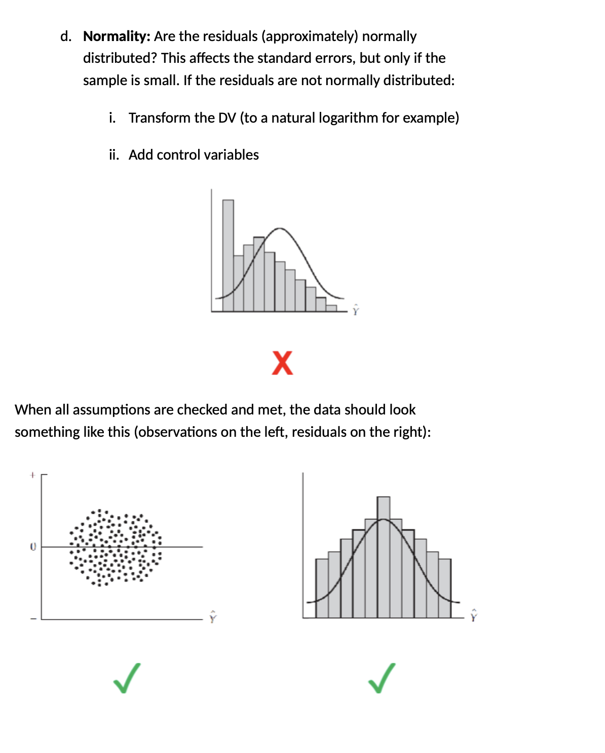
3.Assumptions 

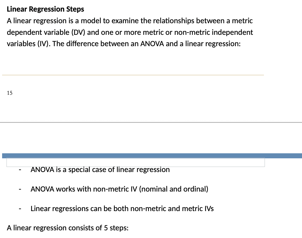
Special cases 

ANOVA is a special case of linear regression.

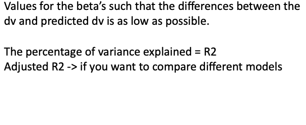
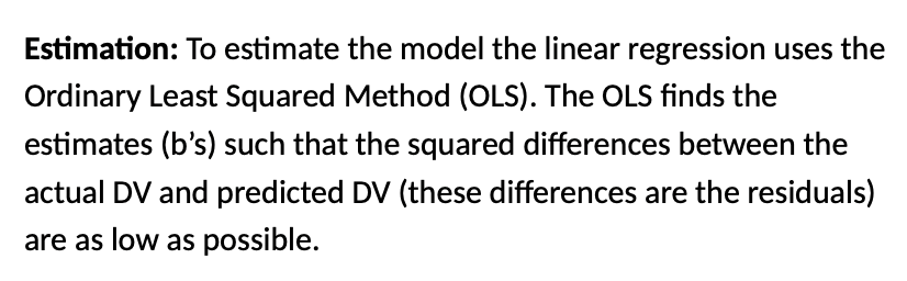
4. Estimating 

Your model guesses sales using a line:

Ŷ = b₀ + b₁X

OLS adjusts b₀ (intercept) and b₁ (slope) until the squared differences between actual sales and predicted sales are minimized.

That’s how it finds the “best fit.”

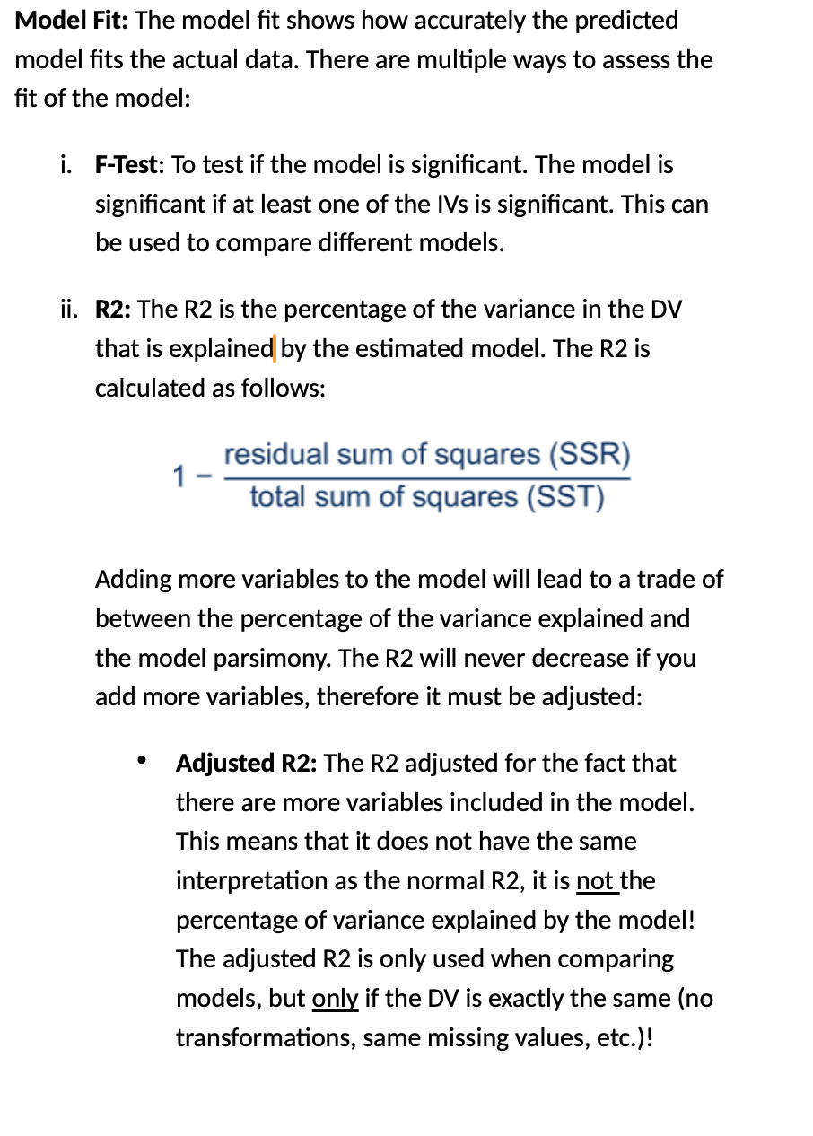
5. Model Fit 

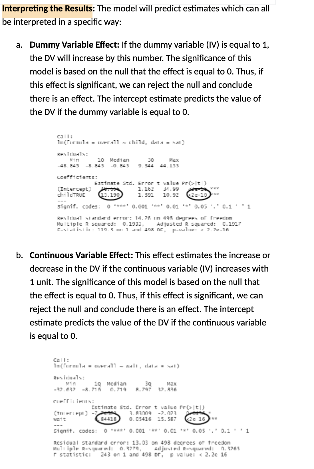
5. Interpreting the Results

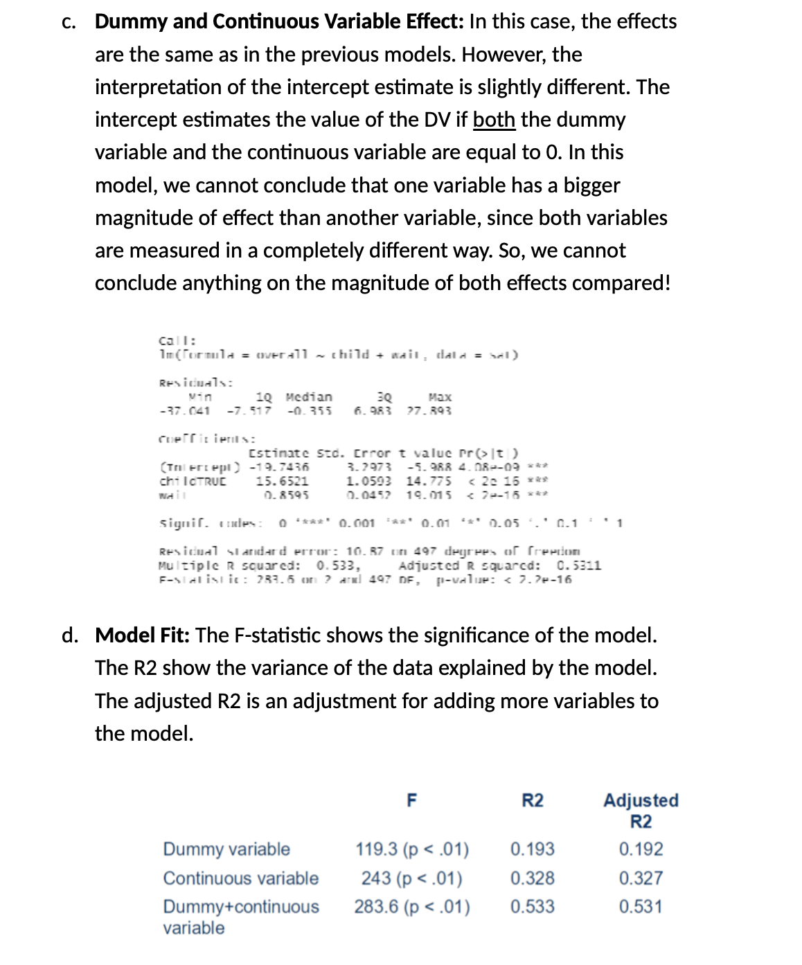
Breaking (The F table ) Down Each Column:1. F-statistic: "Is the model better than nothing?"

• Tests: Whether the model as a whole is significantly better than just using the mean

• All models are significant (p < .01) → All are better than random guessing

• The combined model has the highest F (283.6) → It's the most significantly better than nothing

2. R²: "How much variance does the model explain?"

• Dummy only: 19.3% of satisfaction variance explained by child status

• Continuous only: 32.8% of variance explained by wait time

• Combined: 53.3% of variance explained by both together

• Shows clear improvement with more variables

3. Adjusted R²: "Is the improvement worth the complexity?"

• Notice the pattern: Adjusted R² is slightly lower than R² in each case

• The penalty is tiny because we only added one extra variable

• Key insight: The combined model's adjusted R² (0.531) is still much higher than either single model → Adding wait time was definitely worth it!

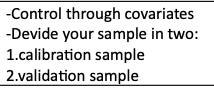
6. Validating outcomes

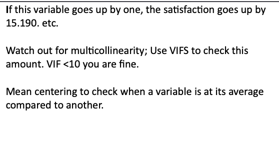
Multicollinearity

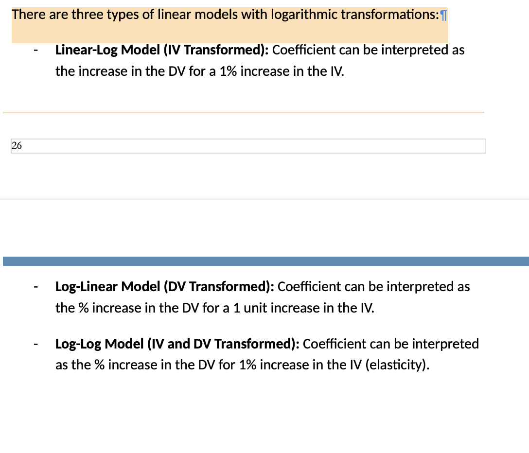
There are three types of linear models with logarithmic transformations: