linear regression

definition

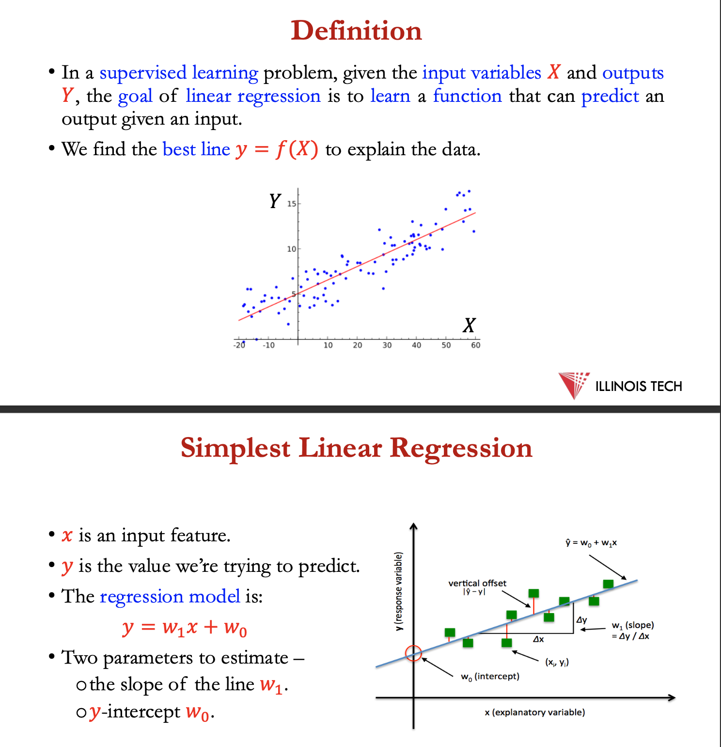
supervised learning problem, given input variables + outputs Y, goal of LR = learn function that can predict an output given an input

• find the best line y = f(X) to explain the data

simplest LR

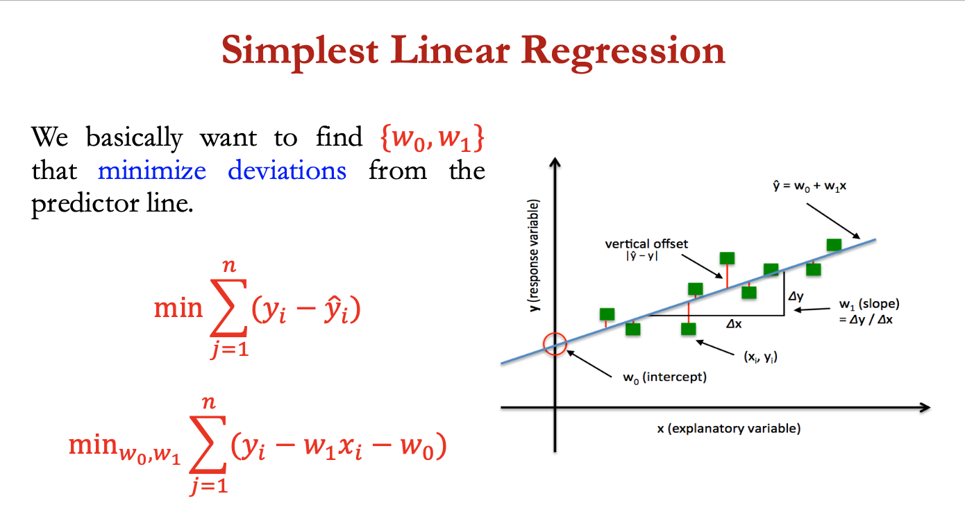
• x = input feature

• y = value we’re trying to predict

• regression model → y = w₁x +w₀

• - 2 parameters to estimate: the slope of the line w₁ and y intercept w₀

basically want to find {w_0, w₁} that minimise derivations from the predictor line

• min w_0,w₁ ∑ (y_i - w₁x_i - w₀)

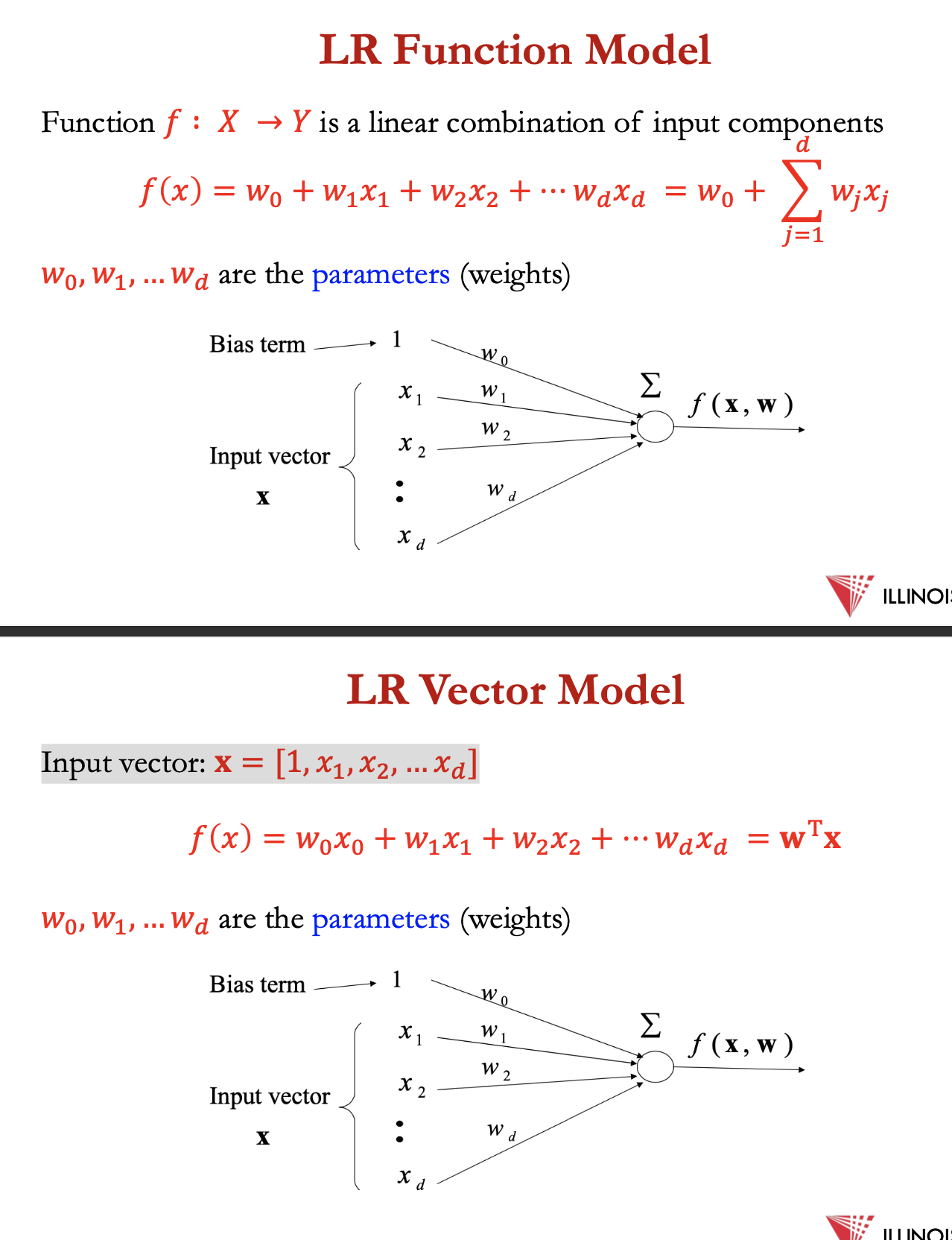
LR function model

function f:  X → Y = linear combo of input components

f(x) = w₀ + w₁x₁   + w₂×₂  + … + w_dx_d = w₀ + ∑   w_jx_j

• w0, w1, wd = parameters (weights)

Input vector: 𝐱 = [1, 𝑥1, 𝑥2, ... 𝑥𝑑]

f(x) =  f(x) = w₀ + w₁x₁   + w₂×₂  + … + w_dx_d = w^Tx

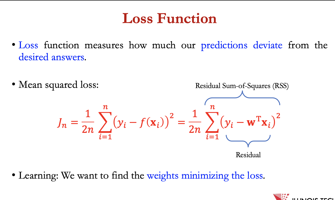
loss func

measures how much out predictions deviate from the desired answers

Mean square loss:

1/2n ∑ (yi - f(xi))² = 1/2n ∑ (yi - w^Txi)²

learning - find weights minimising the loss

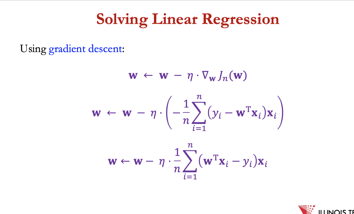
solving LR

using gradient descent:

𝐰←𝐰−𝜂⋅∇ 𝐽_n(𝐰)

𝐰←𝐰−𝜂⋅ (−1/𝑛 ∑ (𝑦𝑖−𝐰^T𝐱𝑖) 𝐱𝑖)

𝐰←𝐰−𝜂⋅1/𝑛 ∑ (𝐰^T𝐱𝑖 −𝑦𝑖) 𝐱𝑖

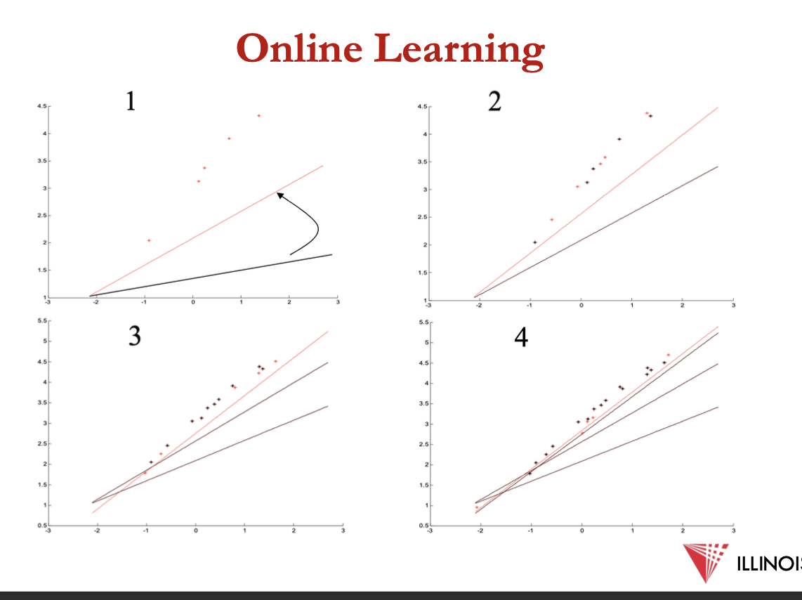
online LR

the loss function defined for the whole dataset for LR =

• 1/2n ∑ (𝑦𝑖 - f(𝐱𝑖))²

online GD - use most recent sample at each iteration

• instead of mean squared loss, use squared loss for individual sample

𝐿𝑜𝑠𝑠_𝑖(𝐰) = ½ ∑ (𝑦𝑖 - f(𝐱𝑖))²

𝐰 ← 𝐰 − 𝜂 ⋅ ∇𝐰 𝐿𝑜𝑠𝑠_𝑖(𝐰)

𝐰←𝐰−𝜂⋅(𝑓(𝐱𝑖) −𝑦𝑖) ⋅𝐱𝑖

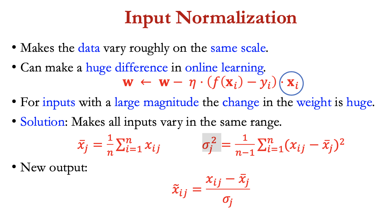
input normalisation

makes data vary roughly on the same scale

• can make a huge diff in online learning

𝐰←𝐰−𝜂⋅(𝑓(𝐱𝑖) −𝑦𝑖) ⋅𝐱𝑖

for inputs w large magnitude, the change in weight = huge

• solution: makes all inputs vary in same range

𝑥 bar j =1/n ∑ xi,j

𝜎² j = 1/ (n-1) ∑ (xij- xbarj)²

new output:

= xij - xbarj / 𝜎j

L1/L2 regularisation

using L1/L2 regularisation, can rewire loss function as:

L_lasso = 1/2n ∑ (yi - f(w^Txi))² + 𝜆 ||w||₁

Bridge = 1/2n ∑ (yi - f(w^Txi))² + 𝜆 ||w||₂²

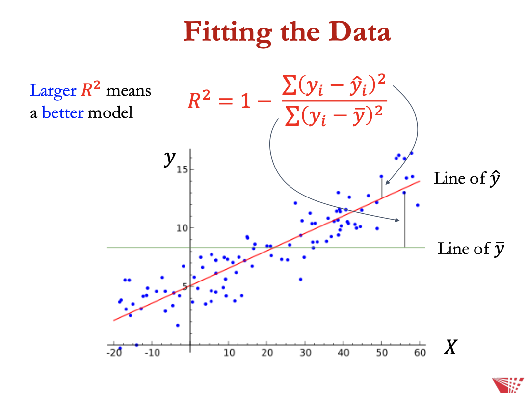
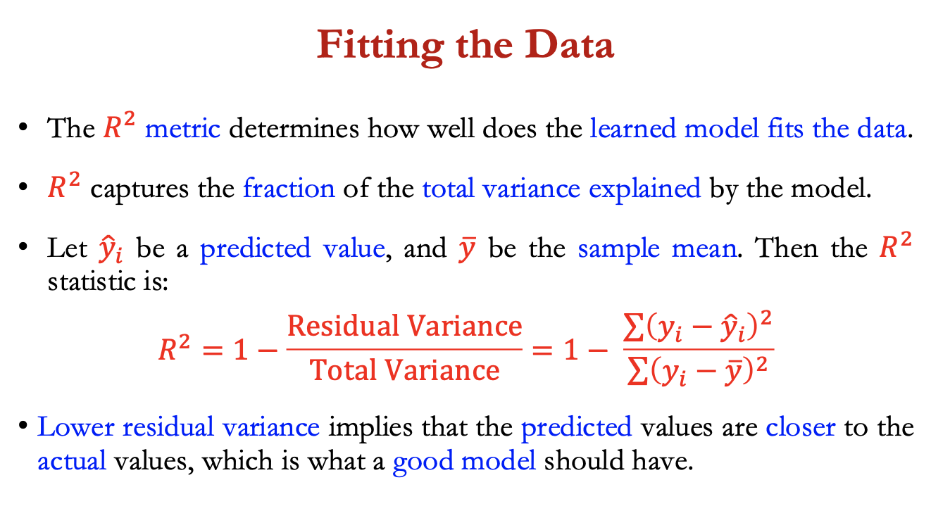
fitting the data

R² metric determines how well the learned model fits the dataa

R² captures the fraction of the total variance explained by the model

let ŷi = predicted value, and y bar = sample mean, R² =

• 1- residual variance/total variance = 1 -  ∑ (yi - ŷi)²/ ∑ (yi - ybar)²

lower residual variance = predicted vans closer to actual values = good model

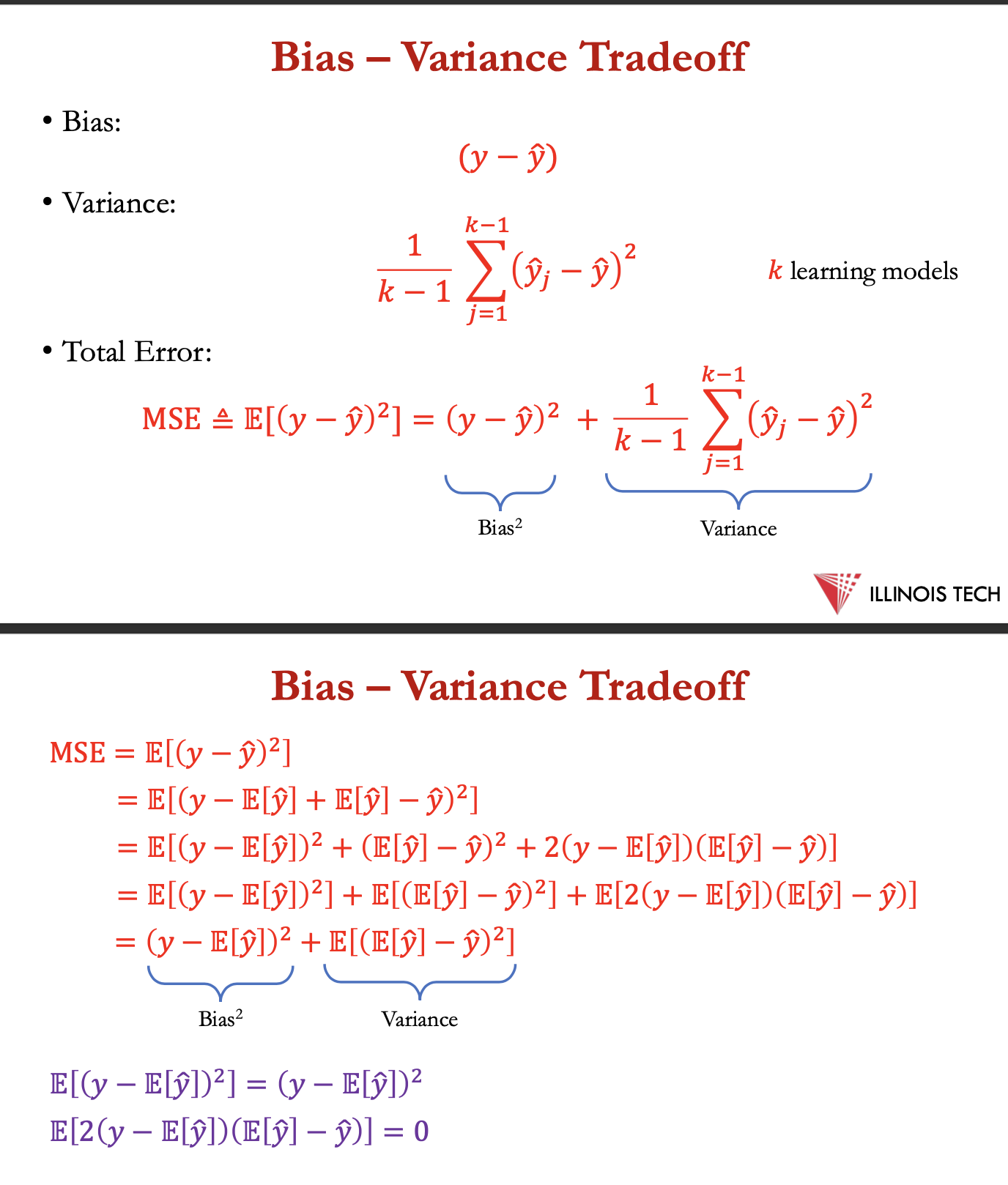
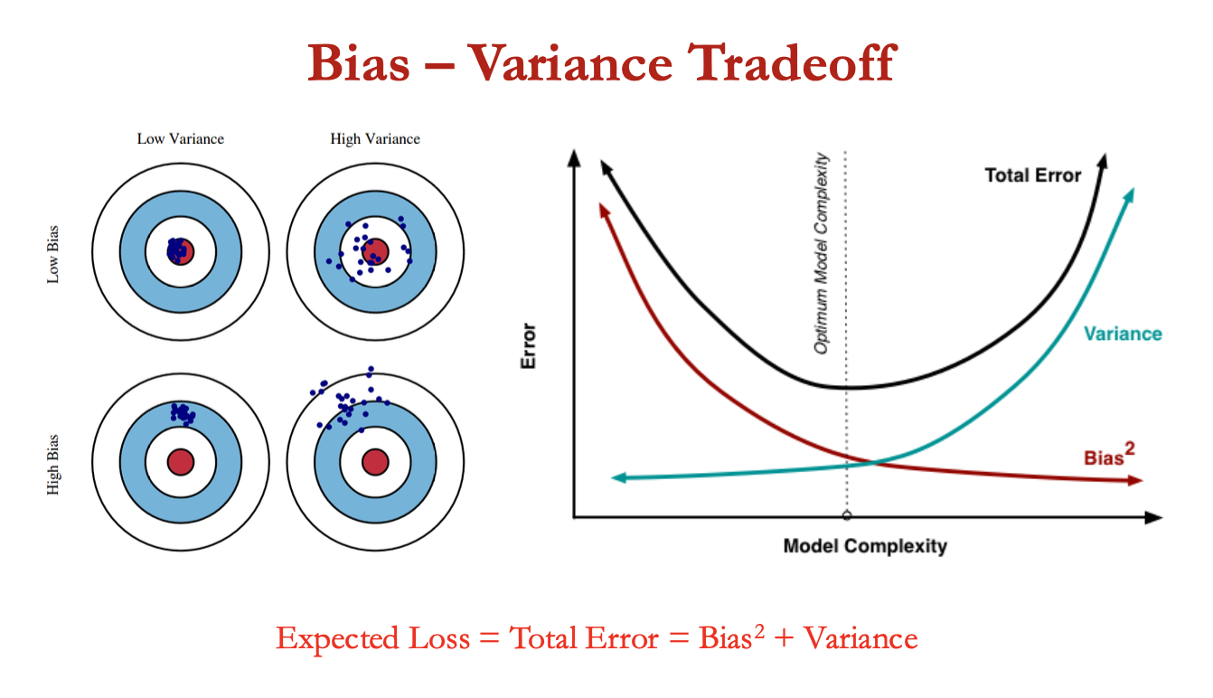
bias variance tradeoff

bias captures inherent error present in model 

• bias error comes from erroneous assumptions in learning algo

bias = contrast between mean prediction of out model + correct prediction

variance captures how much model changes if trained on a diff training set

variance = variation / spread of model prediction values across diff data sampling

bias-variance - conflict in trying to minimise both at same time - these two sources of error that prevent supervised learning algorithms from generalizing beyond their training set

cont

underfitting = model unable to capture underlying pattern of data = high bias + low variance

• when v. less amt of data to build accurate model or linear model used to learn non linear data

overfitting = model captures noise along w the underlying pattern in data

• model is trained a lot over noisy dataset → low bis + high variance

example- predicting price

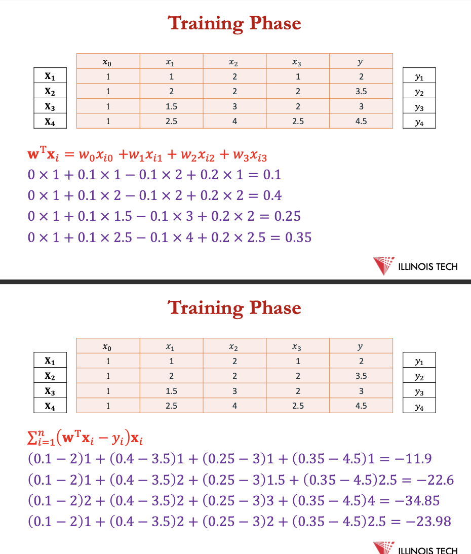
In this dataset, we have 3 input features: Sq ft, Bedrooms, Bathrooms and the output is Price.

• Let us apply linear regression on the price prediction problem, assuming 𝜂 = 0.1 and starting with 𝐰 = [0.0, 0.1, −0.1, 0.2 ]

𝐰←𝐰−𝜂⋅1/𝑛∑ (𝐰^T𝐱𝑖−𝑦𝑖) 𝐱𝑖

𝐰^T𝐱=𝑤0𝑥i0 +𝑤1𝑥i1 +𝑤2𝑥i2 +𝑤3𝑥i3

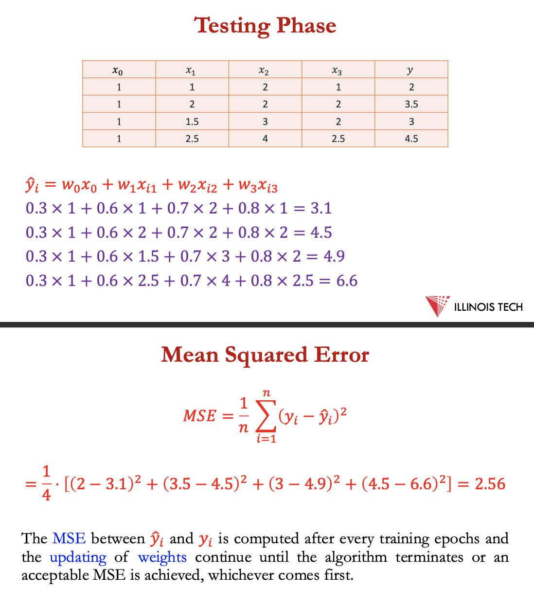
cont - testing + MSE

conclusion

oSimple to implement and easy to interpret.

oComputationally efficient and can handle large datasets effectively.

oIt serves as a good baseline model to compare against more complex regression models.

• Weaknesses:
oUnsuitable for non-linear relationships since it assumes a linear

relationship between variables.

oCan be susceptible to outliers.