Models, Errors and the Normal Distribution

Formula

Error =

Error = Data - Model

𝑒𝑟𝑟𝑜𝑟_𝑖 = 𝑦_𝑖 − ŷ_𝑖

Mode as measuring error

ŷ_𝑖

• The most common value

• A very simplified measure

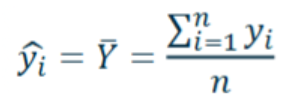
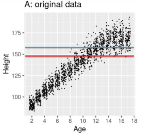
Mean as measuring error

• Summing all data points then dividing by number of data points - Ȳ represents the mean.

• Looks at the average value.

• Poor measure of error - allows values to cancel each other out.

Squared error as measuring error

𝑒𝑟𝑟𝑜𝑟_𝑖 = (𝑦_𝑖 − ŷ_𝑖)²

Can only be positive because you're squaring it.

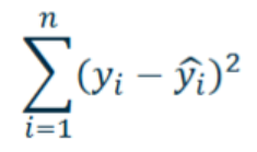
Sum Squared Error (SSE) as measuring error

Sums all of the data points

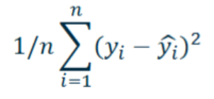
Mean Squared Error (MSE) as measuring error

• Often seen being used in model fitting literature.

• Sum of all the squares divided by number of data points.

• Problem with units being squared.

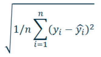
Root Mean Squared Error (RMSE) as measuring error

Unit generated makes the most sense in measuring the model error.

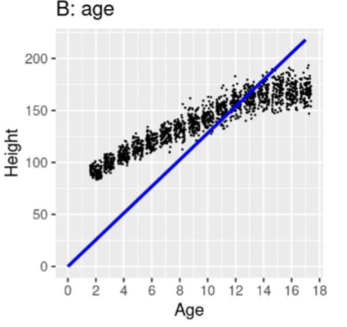
Model A: Judge this model

• Equation: ŷ_𝑖 = B̂_𝑖 ∗ 𝑎𝑔𝑒_𝑖

• Takes into account that there actually are differences across age.

• Model for each data point now depends on age of the specific child, multiplied by a parameter (the slope of the blue line).

• Problem that this model goes through 0 - no child born at 0cm.

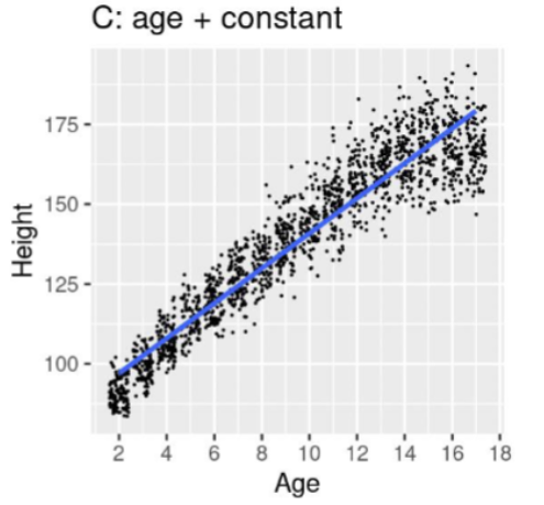
Model B: Judge this model

• Equation: ŷ_𝑖 = B̂₀ + B̂₁ ∗ 𝑎𝑔𝑒_𝑖

• Adds a constant - good job at explaining data, but could be split into other factors.

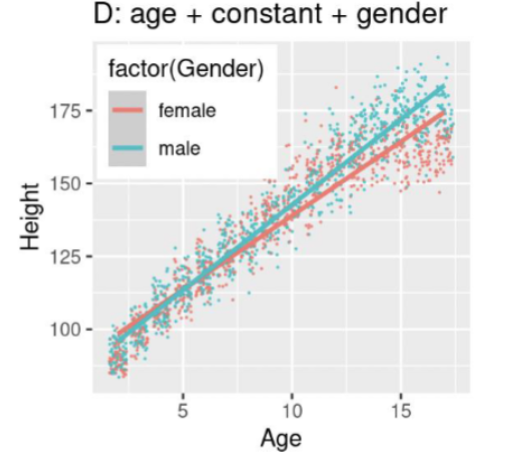
Model C: Judge this model

• Equation: ŷ_𝑖 = B̂₀ + B̂₁ ∗ 𝑎𝑔𝑒_𝑖

• Equation: ŷ_j = B̂₂ + B̂₃ ∗ 𝑎𝑔𝑒_j

• Two separate models.

• Estimating slope and adding a constant for both male and female.

Model D: Judge this model

• ŷ_𝑖 = B̂₀ + B̂₁ ∗ 𝑎𝑔𝑒_𝑖

• ŷ_j = B̂₂ + B̂₃ ∗ 𝑎𝑔𝑒_j

• ŷ_𝑖 = Ȳ

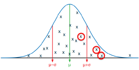
Equation for a normal distribution

𝑁(𝜇, 𝜎²)

𝜇 - specifies where centre of the distribution is placed.

𝜎² - how wide the distribution is.

Likelihood equation

• 𝑃(𝑥|𝜇, 𝜎²)

  • Probability of obtaining a certain value - $x$ - given the two parameters in the model.

  • Circled point closer to the middle - highly likely, compared to lower circled point.

  • Can take all data points and multiply probabilities together to get likelihood of the data set - 𝑃(𝑥₁|𝜇, 𝜎²) * 𝑃(𝑥₂|𝜇, 𝜎²) * 𝑃(𝑥₃|𝜇, 𝜎²)

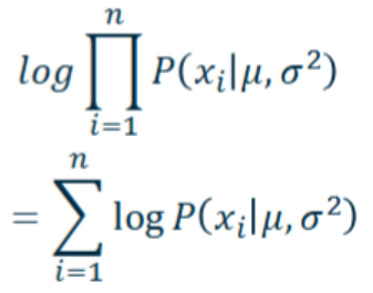
Log likelihood equation

Uses logarithm to describe the likelihood equation

Maximising likelihood = …

Minimising MSE

Minimising MSE = …

Maximising likelihood