International Economics Papers

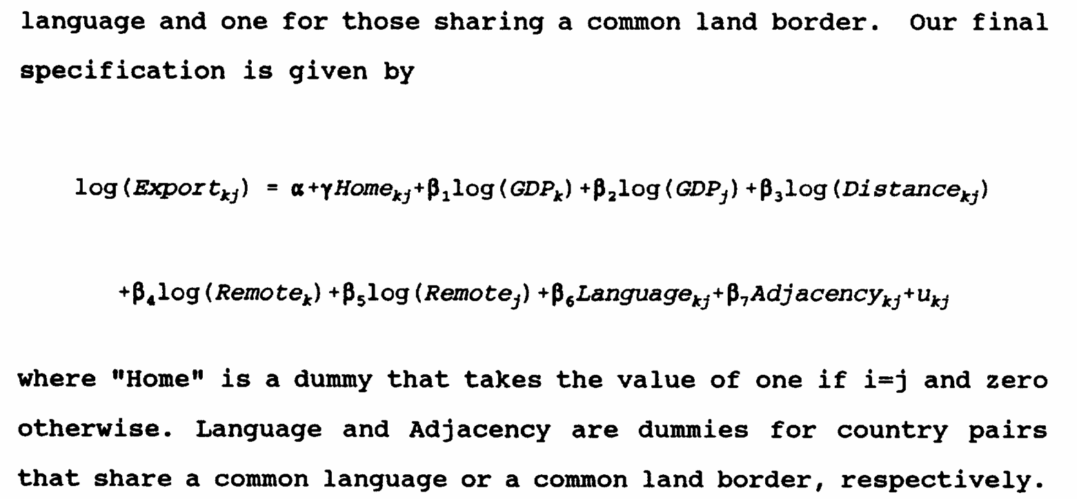
Wolf (1997)

“Patterns of Intra- and Inter-State Trade”

Explores the phenomenon called “home bias.”

Methodology: Gravity model equation with an INTRA-STATE TRADE DUMMY. GDP of states = GSP, distance, and population. Includes remoteness dummy, dummies for adjacency (common border), shared access to the Great Lakes, and joint location on the Atlantic or Pacific coasts. Wolf (1997) treats US states as individual countries (comparables). 1. Same constitution 2. Fixed exchange rate 3. Cultural and institutional homogeneity

Results: There is evidence of home-bias. Intra-state trade is higher than inter-state trade between US states. Therefore, there is home bias not only on an international level, but also on a country level. Robust to sensitivity and different specifications.

Implication: Yes, trade barriers are present, but do not explain the whole story. Something else causes the border effect as well.

What does? Spatial comparative advantage or spatial agglomerations is the answer and explains higher intra-state trade (home bias). Spatial agglomerations increase the border effect since it promotes regional trade. History of accidents in international trade. States located close to each other tend to have similar production patterns and higher trade flows, e.g., the Rust Belt (comparative advantage = specialisation).

What is a spatial agglomeration? Geographic concentration of economic activities, business, or people in a specific area of region (demand externalities and economies of scale), e.g., Silicon Valley

Results (concept explained): Wine (specialised), i.e., cannot choose location of production = more trade since other states cannot produce it, low border effect

Shoes (non-specialised), i.e., produced in each state to save costs of transport = less trade since all states can produce it, higher border effect.

Also, shipment distances are shorter for intermediate goods compared to final goods. Indicates that intermediate goods are more likely to be traded locally, possibly due to the spatial clustering of production stages. States with similar production and trade patterns tend to trade more with each other. However, “specialised” final products are the most traded of them all (wine > shoes).

Wei (1996)

“Intra-National Versus International Trade: How Stubborn are Nations in Global Integration?”

The paper examines the home country bias (we call it the border effect) in the goods market among OECD. All bias needs to come from tariff and non-tariff barriers (and everything that’s not controlled for).

Getting data on intra-national trade flows is challenging. Thus, Wei doesn’t have data on this. Getting bilateral data is easier. Wei (1996) tackled this issue by estimating exports of a country to itself, i.e., EXPORTS (to itself) = GDP (only the goods part, no services) - EXPORTS (to the ROW). Logic: You consume what you don’t export, i.e., export to yourself.

Methodology: Gravity model to estimate the home bias of trade flows. Controls include common language, common border, index of trade openness, remoteness (weighted average of distance from other countries; calculates it different ways and the coefficient is sensitive to methodology), exchange rate volatility, and others. The isolated effect (home bias) captures tariff and non-tariff barriers, and everything that’s not controlled for. Trade flows are estimated for exports to itself (as mentioned above). Also used an IV of population to address potential endogeneity = 2.3x in this specification. Country-specific and country-pair specific fixed effects to control for time-invariant factors, i.e., things that don’t change. FEs are used when examining the effect of integration of the world.

Results: Border effect is 2.5 in the most robust specification, i.e., OECD countries prefer to consume domestic goods 2.5x more than foreign goods (intra-national trade bias). Thus, there is evidence of home bias. Smaller effect than in McCallum US-Canada (1995). It’s 10x for the baseline model in Wei (1996). Exchange rate volatility is not significant, i.e., controlling for volatility doesn’t explain the border effect (home bias). Trade blocks (NAFTA and EU’s EFTA) reduce home bias as integration increases (home bias of 1.7x for EFTA but 2.5x for OECD). However, the evidence is mixed, not very convincing. Sharing a land border (30%) and speaking the same language (80%) increases trade. Lastly, degree of substitutability between goods influences the home bias.

Overall, it’s mostly tariffs, non-tariff barriers, and the degree of substitutability of goods (+common language and common border).

Policy implications: Home bias slowly declines as countries become more integrated (50% decline over the years for EU countries), i.e., the EU Single Market works! EFTA is not as successful as the EU Single Market though. Policies that promote integration are reductions in non-tariff barriers, trade agreements, lower tariffs and regulations, and as people end up having more homogenous preferences due to the Internet.

MRTs from Anderson and Wincoop (2003)

What are Multilateral Resistance Terms?

They solve for omitted variable bias and unobserved heterogenity.

Multilateral resistance terms capture the idea that trade between any two countries is influenced not only by the bilateral trade barriers between them but also by the trade barriers between each of them and all other countries. In other words, the trade flow between country A and country B is affected by how easily country A can trade with other countries and how easily other countries can trade with country B. That is, they capture “remoteness.”

These terms are essentially price indices that reflect the average level of trade barriers faced by each country in its trade with all other countries. They can be thought of as measures of a country's overall trade openness or its integration into the global economy.

MRTs are not observable and need to be estimated.

Alternative approach (FIXED EFFECTS)

Use fixed effects instead of MRTs. It’s easier and does the same job. You can do 1. country specific FE 2. Country-year specific FE (if it’s over multiple periods) 3. Country-pair FE

The choice of fixed effects depends on the nature of the data and the specific research question. Country-specific fixed effects are simpler and control for time-invariant country characteristics, while country-time specific fixed effects account for time-varying factors. Country-pair fixed effects are useful for controlling for pair-specific characteristics in bilateral trade models

McCallum (1995)

"National Borders Matter: Canada-U.S. Regional Trade Patterns"

Examines the home bias within North American (USA and Canada) states and provinces.

Methodology: gravity model approach with GDP, distance, and a dummy of being in the same country (border effect). Creates bilateral pairs (gravity dataset, i.e., destination-origin-time). This time however, it’s only 1988. Heteroscedasticity and the use of OLS.

Data: 1. inter-country trade 2. inter-province trade for Canada 3. no data for inter-state trade for the US. Canada and the US was chosen due to their similarities and high levels of integration.

Tinbergen (1962) and Anderson (1979) wrote about gravity models.

Results: Canadian provinces are 20-times more likely to trade with each other than to trade with US states, i.e., across the border. Sensitivity checks of adding BC dummy confirm it. Thus, the border seems to have an effect on trade even after controlling for GDP, distance, etc. Canada has more West-to-East trade than North-to-South trade, even though Ontario is closer to Michigan than to British Columbia. The gravity model would predict that Ontario will export more to California based on GDP and distance, but that’s not true.

Also, McCallum (1995) isn’t exactly sure what causes the border effect, so further studies by Wei (1996), Chen (2004), and Rauch (1999) look seek to explain the border effect in more detail.

McCallum only covered the year 1988 and argued that a study that covers more years would be necessary. The year when NAFTA came into the effect. Helliwell (1996) extends McCallum’s basic sample to include 1988-1994 and confirms McCallum’s findings, i.e., large home bias even though the US and Canada are an extremely similar country pair.

Anderson and Wincoop (2003): The estimation of the theoretically consistent gravity equation on McCallum’s (1995) data decreases the size of the border effect to 10.7 (as compared to 22). Omitted bias in the original specification, i.e., needed to add MRTs. Also, smaller economies tend to have higher border effects.

Rauch (1999)

"Networks versus Markets in International Trade"

Informal barriers to trade: the role of information costs

Main idea: In matching international buyers and sellers, proximity and common language, and former colonial ties are more important for differentiated products than for homogenous products trade. Therefore, search barriers to trade (information costs) are higher for differentiated products and search costs act as the greatest barrier to trade for differentiated products, i.e., prices are not publicly available.

Why are references prices cheaper? Because you don’t need to advertise them, the price is determined for all commodities, so you just sell it.

His approach: Classifies different goods based on their information costs.

1. References prices on organised exchange (low information costs), e.g., lead or other commodities, easy to match buyers and sellers

2. Reference prices in special magazines/trade publications (medium information costs), e.g., homogenous products like chemicals or other commodities; reference prices distinguish homogeneous from differentiated products

3. Differentiated products (high information costs), e.g., designer shoes, no exchange market

Note: Homogenous commodities are divided into those whose reference prices are quoted on organized exchanges and those whose reference prices are quoted only in trade publications. It’s the same thing, just different medium of exchange.

Method: Estimates 3 different gravity models using the 3 types of goods; GDP, distance, dummies for common border, colonial ties, common language, EEC and EFTA. The expected ranking of coefficients is 1. < 2. < 3. (the highest coefficient on differentiated goods).

Results: Already mentioned above, i.e., common language, colonial ties, and search costs acting as a barrier to trade.

Chen (2004)

"Intra-national versus international trade in the European Union: why do national borders matter?"

Estimates border effects among European Union countries using technical barriers to trade (novel approach) and checks non-trade barriers as well. The exact specification of the gravity equation, together with the choice of the distance measure, are shown to be crucial for assessing the size of the border effect.

Also, Chen (2004) evaluates the determinants of the cross-commodity variation in national border effects. Technical barriers to trade, together with product-specific information costs (Rauch:1999 is correct!), increase border effects, whereas non-tariff barriers are not significant. The spatial clustering of firms is also found to matter (Wolf:1997 is correct too!).

Method: Gravity model of bilateral trade flows (country pair). EU countries are well-integrated and should display low border effects. Estimates the gravity model for both countries and industries, i.e., pooled level, national level and industry level. Uses 2 different measures of distance, i.e., you can calculate distance in better ways that as the crow flies. Wei (1997) did this too. Includes country-specific fixed effects as MRTs to avoid biased estimates. Doesn’t drop zeroes but transforms the data along the lines of Eichengreen and Irvin (1993, 1998). Then, estimated using a Tobit. Hausman test doesn’t show evidence of endogeneity. Non-tariff barriers are expected to display larger border effects because they act as protection from foreign companies (protectionism).

Results: The basic gravity equation estimated with distance, the home coefficient is highly significant, suggesting that an EU country trades about six times more with itself than with a foreign EU country, after adjusting for a number of factors. Sensitive to different measures of distances. Countries that joined the EU later or are smaller have the highest border effect coefficients. Border effects also differ across industries (easier to transport have lower and vice versa). Industries with no TBTs, or with TBTs removed, display smaller border effects (hypothesis of technical barriers to trade confirmed!). The positive but insignificant coefficient on the interaction term implies that non-tariff barriers do not matter in explaining border effects, a finding consistent with that by Head and Mayer (2000). Chen (2004) confirms Wolf (1997), i.e., spatial agglomerations increase the border effect (countries group together and don’t have a need to trade across the border). Also, the findings are consistent with Rauch (1999), i.e., information costs increase the border effect meaning that higher costs cause consumers to favour domestic alternatives.

Overall, border reduce trade. There is empirical evidence that supports it.

Technical barriers to trade, together with product-specific information costs, are shown to increase border effects. Non-tariff barriers are not significant. Our analysis further suggests that the elasticity of substitution among varieties is not driving the cross-industry variance in border effects. Finally, cross-border transaction costs may lead some firms to agglomerate, so that industries not tied to a specific location display larger border effects. This can be taken as an indication that border effects are, to some extent, endogenous.

Policy implications: In the context of the European Union’s integration process, what can be said about the evolution of border effects? With the 1992 Single Market Programme, the abolition of border controls on intra-EU trade, as well as the harmonization or mutual recognition of standards and other regulations, were intended to increase intra-EU competition and hence intra-EU trade. Accordingly, and as suggested by our results relating to TBTs, further market integration should reduce the magnitude of border effects. Monetary Union should also stimulate intra-EU trade and reduce border effects by increasing transparency between markets (Heskel and Wolf; didn’t work actually). Border effects can therefore be expected to decrease in the future but given that they also reflect the optimal location choices of producers, it seems unlikely that they will fully disappear.

The Border Effect Puzzle

Understanding the border effect is important for welfare implications.

National trade barriers (tariffs, quotas, exchange rate variability, transaction costs, different standards and customs, regulatory differences, etc.) appear as obvious candidates in causing the volume of domestic trade to exceed that of international trade since they increase the transaction costs for shipments crossing borders. However, although this trade barrier explanation is very attractive, the few papers which attempt to explain border effects by (border related) trade barriers generally find poor evidence in favour of the hypothesis (Wei, 1996; Hillberry, 1999; Head and Mayer, 2000).

A second explanation could therefore be that intermediate and final goods producers agglomerate in order to avoid trade costs, reducing the need for cross-border trade (Wolf, 1997; Hillberry, 1999; Hillberry and Hummels, 2000). Note that the two explanations are not mutually exclusive, and it could well be that both contribute to the overall effect.

The size of the effect is also a subject of multiple debates, i.e., 20x higher domestic trade is too high (McCallum, 1995). Anderson and Wincoop (2003) find around 10x.

Wei (1996) examines whether the impact of borders can be attributed to exchange rate volatility between OECD countries, but finds no significant effect. Head and Mayer (2000) show that non-tariff barriers do not explain border effects in Europe. Hillberry (1999) investigates the role of trade policy (tariffs), regulations, information and communication costs (captured by the extent of multinational activity), product-specific information costs, public procurement and hysteresis in domestic transportation networks, but none of these appears significant in explaining border effects. Also, it is more costly to obtain some information about the quality, or even the existence, of a foreign product as compared to a domestic product, we would expect this higher cost to reduce the quantities of foreign goods purchased (Rauch, 1999), and hence to contribute to the existence of border effects. Wolf (1997) shows that spatial agglomerations contribute to trade barriers. Hillberry (1999) and Hillberry and Hummels (2000) also show that the spatial clustering of firms magnifies border effects.

Chen (2004): Industries with no TBTs, or with TBTs removed, display smaller border effects (hypothesis of technical barriers to trade confirmed!). The positive but insignificant coefficient on the interaction term implies that non-tariff barriers do not matter in explaining border effects, a finding consistent with that by Head and Mayer (2000). Chen (2004) confirms Wolf (1997), i.e., spatial agglomerations increase the border effect (countries group together and don’t have a need to trade across the border). Also, the findings of Chen (2004) are consistent with Rauch (1999), i.e., information costs increase the border effect meaning that higher costs cause consumers to favour domestic alternatives.

Overall, border reduce trade. There is empirical evidence that supports it.

Chen (2004) and technical barriers to trade

Member states can restrict intra-EU imports on the grounds of health, safety, environmental and consumer protection. These obstacles, known as technical barriers to trade (TBTs), impose some additional costs on exporters who want to access foreign markets, and could hence contribute to border effects. Various measures were implemented in order to remove these barriers13, but in 1996, about 79% of intra-EU goods trade were still affected by TBTs (European Commission, 1998).

Chen (2004): We expect those industries with no TBTs, or with TBTs removed, to display smaller border effects.

Policy implications for trade and the border effect

From Chen (2004)

Policy implications: In the context of the European Union’s integration process, what can be said about the evolution of border effects? With the 1992 Single Market Programme, the abolition of border controls on intra-EU trade, as well as the harmonization or mutual recognition of standards and other regulations, were intended to increase intra-EU competition and hence intra-EU trade. Accordingly, and as suggested by our results relating to TBTs, further market integration should reduce the magnitude of border effects. Monetary Union should also stimulate intra-EU trade and reduce border effects by increasing transparency between markets (Haskel and Wolf 1999; didn’t work actually). Border effects can therefore be expected to decrease in the future but given that they also reflect the optimal location choices of producers, it seems unlikely that they will fully disappear.

Engel and Rogers (1996)

"How Wide Is the Border?" (Provides a measure of how important the border is relative to distance; we call it the width of the border.)

Examines the deviations from the law of one price (LOOP) using CPI data for 23 U.S. and Canadian cities across 14 categories of consumer prices. The study investigates the role of distance and national borders in explaining the variation in prices of similar goods in different cities, e.g., sticky prices, integration of labour markets, transportation costs, and trade barriers

Main hypothesis: The volatility of price of similar goods between cities should be positively related to the distance between those cities; but when we hold distance constant, volatility should be higher between two cities separated by the national border.

Method: gravity-type framework with a dummy if cities are in different countries; US and Canada are chosen due to their similarity, e.g., culture, common language, preferences, and since they share a border. 23 cities in Canada and the US, then create city pairs.

Important considerations behind the failure of the LOOP: Mark-up, i.e., pricing-to-the market may be responsible for the failure. Transportation costs and trade barriers, e.g., tariffs. Different wages and cost of labour. Better or worse integration in domestic markets compared to foreign markets. Sticky prices due to the currency, e.g., menu costs or contracts, or simply currency fluctuations.

Results: The distance between cities explains a significant amount of the variation in the prices of similar goods in different cities, i.e., distance has a positive effect on price dispersion in all regressions and is generally significant for all types of goods. The variation is much higher for two cities separated by national border than for two cities in the same country (more volatile prices across the border than within a country). However, the distance alone doesn’t explain it, so the border dummy matters. The border dummy is positive and significant in all cases. Crossing a border is equivalent to 1780 miles of distance between two cities (in the same country). Sticky nominal prices are one explanation, but don’t explain most of the border effect. The failure of the LOOP also affects the behaviour of real exchange rates. Also, the failure of the LOOP means that markets are not perfectly integrated. Adds wage volatility to test the hypothesis of more homogenous labour markets within a country = no effect on the border effect, only on distance, i.e., labour markets further apart are less integrated. Even if we exclude nominal exchange rates, the border still matters.

Final results and proportions:

Border effect = 18.9%-33.3% of the standard deviation in cross-border prices (depends on the specification). Sticky prices are responsible for this difference (around 33% of the border puzzle). Index of relative prices, i.e., some cities are more expensive that others for logical reasons, explain a part of it too. Formal trade barriers may not fully explain it, but informal barriers are significant. Wage costs do not explain the border effect.

Distance = 20.3% of total price dispersion.

Overall, sticky nominal prices, e.g., menu costs and contracts, explain most of the border effect, but not all. A portion of it remains unexplained. Possibly due to demand elasticities or homogeneity of productivity shocks in non-tradeable sectors (the paper doesn’t test these).

And yes, the border and distance matter in explaining different prices, i.e., the failure of the LOOP, in addition to commonly known factors like mark-ups (price discrimination).

The results confirm McCallum’s (1995) findings that despite the relative openness of the US-Canada border, the markets are still segmented.

Rogoff (1996)

"The Purchasing Power Parity Puzzle"

The paper covers the lore of testing for PPP, i.e., 4 different approaches over the years, each being more advanced. They want to reject the Random Walk hypothesis and prove that PPP converges, but initial tests have weak explanatory power. You test for it using a unit root, i.e., you want no unit root = stationary. Test for stationarity is ADF test.

PPP = once converted to a common currency, prices should be equal

1.Convergence to PPP is extremely slow (15% per year; 3-5 half-life). 2.Short-run deviations from PPP are large and volatile.

What is the PPP Puzzle? “Why do real exchange rates fluctuate wildly in the short term, but take a long time to settle after a shock?”

Most evidence explaining short-term exchange rate volatility points to changes in portfolio preferences, short-term asset bubbles, and monetary shocks. Such shocks affect the real economy, but prices and wages are sticky in the short run.

LOOP = P = eP* ; the same concept as PPP, just on a micro scale, i.e., when prices of a specific good are converted to a common currency, the same good should sell for the same price in different countries. Tariffs, transportation costs and non-tariff barriers create price differences and make the LOOP not hold. The tradability of a good matters too, i.e., non-tradable goods can have different prices (Big Mac Index).

Why are prices of Bic Macs different? 1. Non-tradable inputs, e.g., labour and restaurants 2. Taxes are different 3. Profit margins due to competition 4. Bundles and regional prices, e.g., ketchup is free in the US, but not in Europe

The LOOP can hold very well for some commodities, such as gold. The LOOP deviations are highly correlated with exchange rate movements (Knetter, 1989; studied German beer shipped to the UK and vice versa). Engel and Rogers (1995) show that prices are a function of distance and border, but the border effect has a disproportionally stronger effect on prices, i.e., within a country prices are different that cross country prices.

Why don’t international prices converge? 1. Local distribution costs (transportation costs, taxes and wages), i.e., the non-tradable component 2. Trade barriers, non-trade barriers, and regulations. 3. Technical barriers, e.g., local electricity standards (120V 60Hz) 4. Mark-ups and price discrimination

Absolute and Relative PPP. 1. Baskets of goods (CPI) are different across countries, e.g., Japan with fish, Hungary with meat. 2. CPI is an index, not an absolute measure of prices, i.e., base years may vary, and we must assume that the absolute PPP help in a specific year. 3. Absolute CPI is hard to collect and has limitations.

1.Long-run convergence to PPP (Random Walk) Simple test for unit root

Empirically, the PPP fails in the short run due to sticky prices and wages, while the real and nominal exchange rates change in the short run. This is directly related to Dornbush (1976) and the model of overshooting, i.e., the Dornbusch model explains why the PPP fails in short run. However, evidence shows that even after a year or two, PPP doesn’t converge back. Why? Real exchange rates of major currencies likely follow a random walk (failed to reject the hypothesis), which explains why there is no convergence in the long run.

2.Better tests based on long-horizon datasets; Test for unit root unit using a long-term dataset.

Frankel (1986) argued that the reason for failure to reject the random walk model was due to a lack of power, i.e., you need longer datasets to see it. Often decades. Therefore, Frankel (1986) was able to reject the random walk hypothesis and conclude that half-life of PPP is 4.6 years (decay of 15% per year). However, it depends on a specific currency, a set of countries, and time period. Nevertheless, there is strong evidence of convergence of PPP in the long run (half-life of 3-5 years).

3.Long-term dataset with addition of more countries; Test for unit root using a long-term dataset and multiple countries

Adding more countries (over 150) enhanced the explanatory power of a unit root test. Frankel and Rose (1995) are able to reject the random walk model and find a half-life of around 4-5 years, which is in line with previous studies. One criticism is that high inflation countries upward bias the mean reversion, i.e., faster convergence due to higher volatility of currency.

There is evidence of non-linearities, i.e., converges at a decreasing rate, especially fast if initial shock is large.

3.x Modifications to PPP: 3 modifications in total, but the Balassa-Samuelson Hypothesis is the most famous one.

In B-S, rich countries tend to have higher price levels than poor countries (when everything is converted to a common currency). Why? Rich countries are more productive in the tradable goods sector due to superior technology. There is little to no difference in productivity in non-tradable sectors. Productivity = wages. However, wages are the same in all sectors, so the country’s CPI must rise. The B-S model also expects real currency appreciation for more productive economies, but there’s mixed empirical evidence of this, e.g., works for Japan (Yen appreciated in the 1970s) but doesn’t hold for all currencies. Nevertheless, economists generally agree that the B-S hypothesis holds when using long-horizon datasets and including multiple countries, e.g., Japan’s example.

4.TAR model (Threshold autoregressive); Test for non-linearities. Not mentioned in Rogoff (1995), but it’s the most modern and promising approach

Also tests for a unit root, but in a more accurate manner. Transaction costs are non-linear, so deviations from the LOOP should contain non-linearities. Thus, we test for these non-linearities using a TAR model, i.e., when the LOOP is outside the threshold, arbitrage by travelling to a different district become profitable, which causes prices to adjust and converge back. Outside of band = PPP/LOOP holds due to arbitrage. Inside=doesn’t hold due to no arbitrage (not worth it).

In conclusion, international markets although integrated, remain very segmented due to 1. transportation costs 2. tariff and non-tariff barriers 3. information costs 4. lack of labour mobility. Thus, domestic markets are better integrated than international markets, meaning that there are going to be greater differences in international prices than in regional prices.

Haskel and Wolf (1999)

IKEA: "Why Does the 'Law of One Price' Fail? A Case Study"

Uses individual retail prices in IKEA to examine the extent and permanence of violations of the LOOP for identical products sold in different countries. Data collection via regional catalogues since all products are identical and tradable.

Using a CPI is not ideal due to being 1. too broad 2. different baskets of goods 3. base years. Using individual prices may be better if goods are 1. tradable 2. identical. IKEA furniture matches that description.

After looking at the data for the first time, they find median deviations of 20–50%. Then, they try to understand what causes the failure of the LOOP and come up with this: The differences are not systematic across very similar goods within a product group (e.g. two types of mirrors), nor across product groups, meaning that local distribution costs are not responsible for violations of the LOOP and pointing instead to differences in mark-ups (3rd degree price discrimination), i.e., managers face different competitive pressures and need to adjust specific prices to meet the regional demand.

Moreover, they add controls for common language, common border, EU Single Market, i.e., high integration, and find that more integrated countries display smaller price differences. That’s because arbitrage can influence, i.e., lower, prices. People travel across the border, which decreases price differences and leads to convergence. Countries that are further apart have higher price differences, i.e., arbitrage not possible. Related to the TAR model (non-linearity test).

Also mentioned in the paper: A common currency does not significantly help with price convergence / full price transparency. The ECB assumed that a common currency would lead to price transparency in the EU. It didn’t!

Conclusion: The final retail price is a product of: 1. import price (production cost) = not significant 2. local distribution costs (transport + wages) = not significant 3. mark-up (determined by managers and driven by local trends and competition) = significant and response for the failure of the LOOP!

Evidence of arbitrage and price convergence in highly integrated countries that share a border, e.g., Slovakia and Hungary. Also, competitive pressures reduce prices. However, idea has different market power in different countries, which allows them to set prices in some regions.

Method: gravity-like approach with country-pairs, market size, distance, population, common language, and common border controls.

Policy implications: Highly integrated markets have lower price divergence, but it doesn’t lead to price transparency as the ECB hoped for. Competitive pressures limits price divergence, i.e., IKEA not having too much market power to set their own prices.

Head and Mayer (2000)

Non-tariff barriers, e.g., quotas, licensing requirements, are not significant in explaining the border effect.

Technical barriers to trade are safety regulations, environmental restrictions, and other technical aspects.

Technical barriers to trade are a subset of non-tariff barriers.

Hillbery (1999)

Different types of trade barriers, e.g., regulations, trade policy, is not significant in explaining the border effect.