Stats Exam #2 (Ch 5-8)

random variable

a numerical description of the outcome of an experiment

discrete random variable

may assume either a finite number of values or an infinite sequence of values

continuous random variable

may assume any numerical value in an interval or collection of intervals

probability distribution

for a random variable, describes how probabilities are distributed over the values of the random variable

• can describe a discrete one w a table, graph, or formula

two types of discrete probability distributions

1. uses the rules of assigning probabilities to experimental outcomes to determine probabilities for each value of the random variable

2. uses a special math formula to compute the probabilities for each value of the random variable

probability function (discrete prob dist)

provides the probability for each value of the random variable

• f(x) > or = 0

• sum of f(x) = 1

several discrete probability distributions specified by formulas

• discrete-uniform

• binomial

• poisson

• hypergeometric

• in addition to tables and graphs, a formula that gives the probability function, f(x), for every value of x is often used to describe the probability distributions

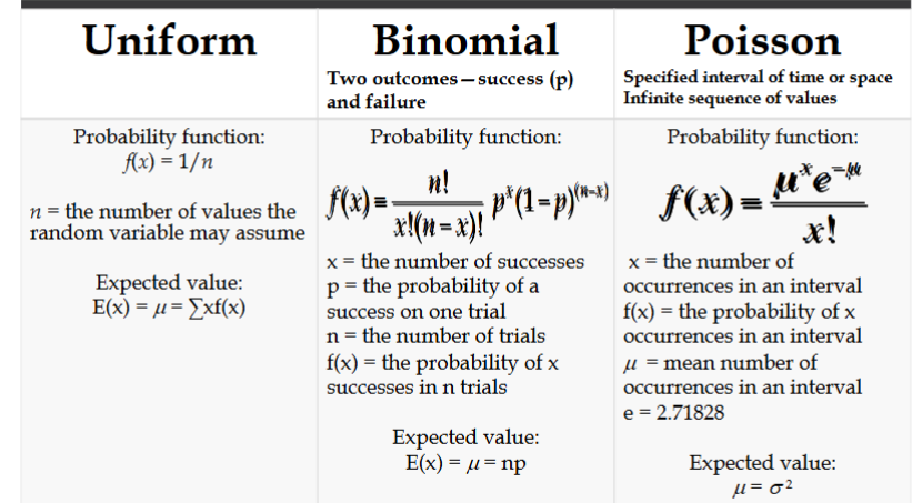
discrete uniform probability distribution

• the simplest example of a discrete probability distribution given by a formula

• f(x) = 1/n

• n is the number of values the random variable may assume (the values of the random variable are equally likely)

expected value

• mean of a random variable, is a measure of its central location

• a weighted average of the values the random variable may assume. the weights are the probabilities

• does not have to be a value the random variable can assume

variance

summarizes the variability in the values of the random variable

• sigma squared

• a weighted average of the squared deviations of a random variable from its mean

• the weights are the probabilities

standard deviation

• sigma

• the positive square root of the variance

four properties of a binomial experiment

1. the experiment consists of a sequence of n identical trials

2. two outcomes, success and failure, are possible on each trial

3. the probability of a success, denoted by p, does not change from trial to trial (stationarity assumption)

4. the trials are independent

binomial probability distribution

• our interest is in the # of successes occurring in n trials

• we let x denote the # of successes occurring in n trials

• =binom.dist

expected value (binomial dist)

E(x) = u = np

variance (binomial dist)

np (1-p)

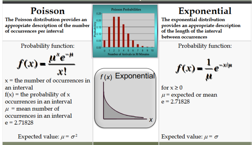
poisson probability distribution

• random variable is often useful in estimating the # of occurrences over a specified interval of time or space

• it is a discrete random variable that may assume an infinite sequence of values (x = 0,1,2,….)

• ex:

  • # of knotholes in 14 linear feet of pine board

  • # of vehicles arriving at a toll booth in one hour

• specified interval of time or space. infinite sequence of values

two properties of a poisson experiment

1. the probability of an occurrence is the same for any two intervals of equal length

2. the occurrence or nonoccurrence in any interval is independent of the occurrence or nonoccurrence in any other interval 

• mean and variance are equal

poission probability function

• since there’s no stated upper limit for the # of occurrences, the probability function f(x) is applicable for values x= 0,1,2… w out limit

• in practical applications, x will eventually become large enough so that f(x) is approximately zero and the probability of any larger values of x becomes negligible

• = poisson.dist

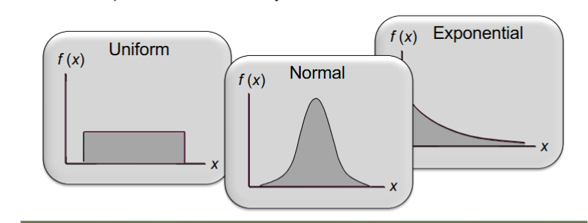
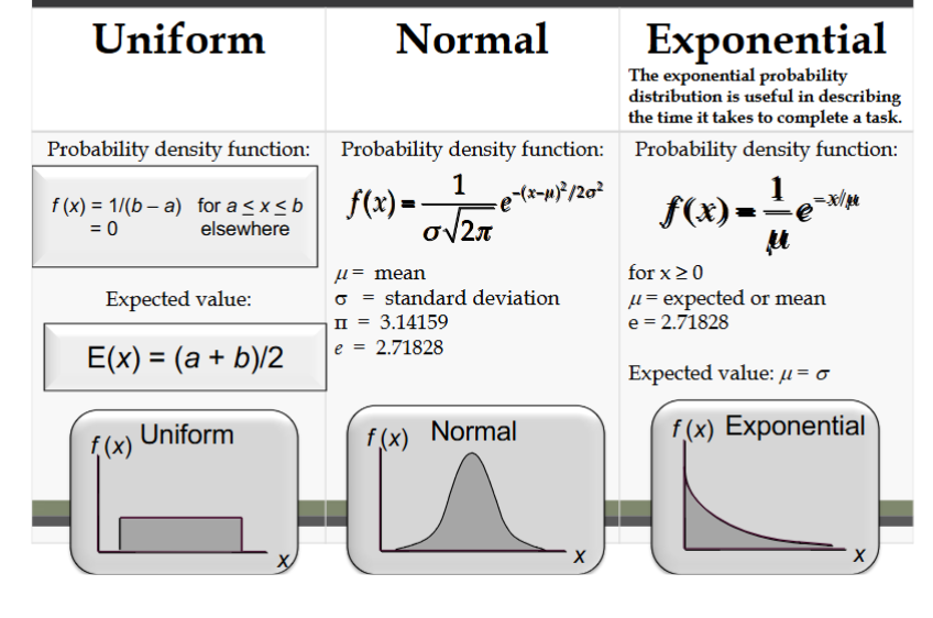
types of continuous probability distributions

• uniform probability distribution

• normal probability distribution

• exponential probability distribution

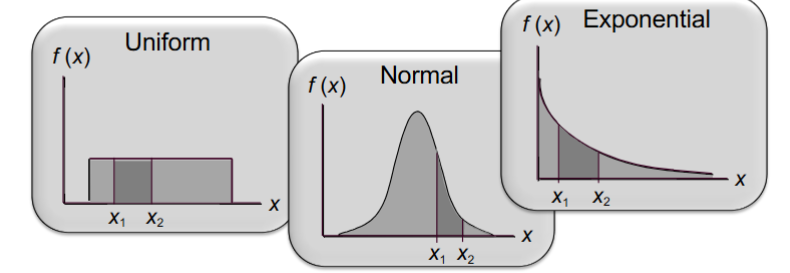
continuous random variable

• can assume any value in an interval on the real line or in a collection of intervals

• it’s not possible to talk about the probability of the random variable assuming a particular value

• instead, we talk about the probability of the random variable assuming a value w in a given interval

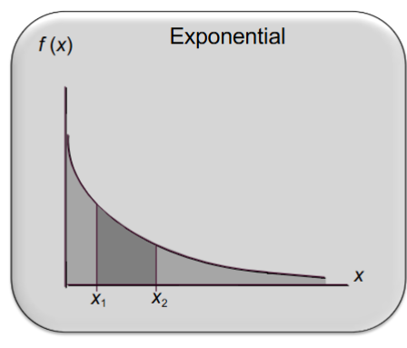
• the probability of the random variable assuming a value w in some given interval from x1 to x2 is defined to be the area under the graph of the probability density function btw x1 and x2

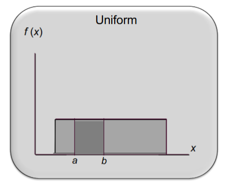
uniform probability distribution

• a random variable is uniformly distributed whenever the probability is proportional to the interval’s length

• probability density function: 

  • f(x) 1/(b-a)

  • a is the smallest value the variable can assume

  • b is the largest value the variable can assume

expected value & variance of x for uniform probability distribution

• E(x) = (a+b)/2

• Var(x) = (b-a)²/12

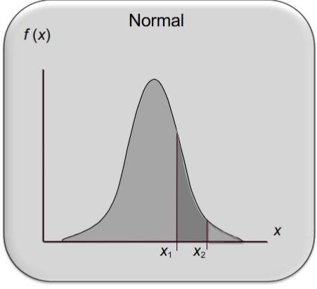
area as a measure of probability

• the area under the graph of f(x) and probability are identical

• this is valid for all continuous random variables

• the probability that x takes on a value btw some lower value x1 and some higher value x2 can be found by computing the area under the graph of f(x) over the interval from x1 to x2

normal probability distribution

• the most important distribution for describing a continuous random variable

• widely used in statistical inference

• ex:

  • heights of ppl

  • rainfall amounts

  • test scores

  • scientific measurements

• doctrine of chances Abraham de Moivre

normal probability distribution characteristics

• the distribution is symmetric; its skewness measure is zero 

• the entire family of normal probability distributions is defined by its mean u and its standard deviation sigma

• the highest point on the normal curve is at the mean, which is also the median and mode

• the mean can be any numerical value: negative, zero, or positive 

• the standard deviation determines the width of the curve: larger values result in wider, flatter curves

• probabilities for the normal random variable are given by areas under the curve. the total area under the curve is 1 (0.5 to the left of the mean and 0.5 to the right)

• empirical rule:

  • 68.26% of values ±1

  • 95.44% of values ±2

  • 99.72% of values ±3

standard normal probability distribution characteristics

• a random variable having a normal distribution w a mean of 0 and a st dev of 1 is said to have a standard normal probability distribution

• the letter z is used to designate the st normal random variable

• we can think of z as a measure of the # of st dev away from mean

z-score

• standardized value

• it denotes the number of st dev a data value xi from the mean

• =standardize

excel for normal distributions

• norm.s.dist is used to compute the cumulative probability given a z value

• norm.s.inv is used to compute the z value given a cumulative probability

• the s reminds us that they relate to the standard normal probability distribution

• norm.dist is used to compute the cumulative probability given an x value

• norm.inv is used to compute the x value given a cumulative probability

exponential probability distribution

• useful in describing the time it takes to complete a task

• ex:

  • time btw vehicle arrivals at a toll booth

  • time required to complete a questionnaire

  • distance btw major defects in a highway

• in waiting line applications, the exponential distribution is often used for service times

• mean and st dev equal

• skewed right w a measure of 2

excel exponential probabilities

• expon.dist function can be used to compute exponential probabilities

• 3 arguments: 

  • 1st : the value of the random variable x

  • 2nd: 1/u (the inverse of the mean # of occurrences in an interval)

  • 3rd: true or false (always true)

relationship btw the poisson and exponential distributions

• the poisson distribution provides an appropriate description of the # of occurrences per interval

• the exponential distribution provides an appropriate description of the length of the interval btw occurrences

discrete probability distributions summary

continuous probability distributions summary

element

the entity on which data are collected

population

a collection of all the elements of interest

sample

subset of the population

sampled population

the population from which the sample is drawn

frame

a list of the elements that the sample will be selected from

the reason we select a sample:

• to collect data to answer a research question about a population

• the sample results provide only estimates of the values of the population characteristics

• the reason is simply that the sample contains only a portion of the population

• with proper sampling methods, the sample results can provide “good” estimates of the population characteristics

finite populations

• defined by lists such as:

  • organization membership roster

  • credit card account numbers

  • inventory product numbers

• a simple random sample of size n from a finite population of size N is a sample selected such that each possible sample of size n has the same probability of being selected

sampling with replacement

replacing each sampled element before selecting subsequent elements

sampling without replacement

the procedure used most often

in larger sampling projects…

computer-generated random numbers are often used to automate the sample selection process

sampling from an infinite population

• sometimes we want to select a sample, but find it’s not possible to obtain a list of all elements in the population

• as a result, we can’t construct a frame for the population

• hence, we cannot use the random number selection procedure

on-going process

• populations are often generated by an ongoing process where there is no upper limit on the # of units that can be generated

• some examples of on-going processes, with infinite populations, are:

  • parts being manufactured on a production line

  • transactions occurring at a bank

  • telephone calls arriving at a technical help desk

  • customers entering a store

a random sample from an infinite population

• is a sample selected such that the following conditions are satisfied

  • each element selected comes from the population of interest

  • each element is selected independently

• in the case of an infinite population, we must select a random sample in order to make valid statistical inferences about the population from which the sample is taken

point estimation

• a form of statistical inference

• we use the data from the sample to compute a value of a sample statistic that serves as an estimate of a population parameter

• point estimator

target population

the population we want to make inferences about

sampled population

the population from which the sample is actually taken

• whenever a sample is used to make inferences about a population, we should make sure that the targeted population and the sampled population are in close agreement

process of statistical inference

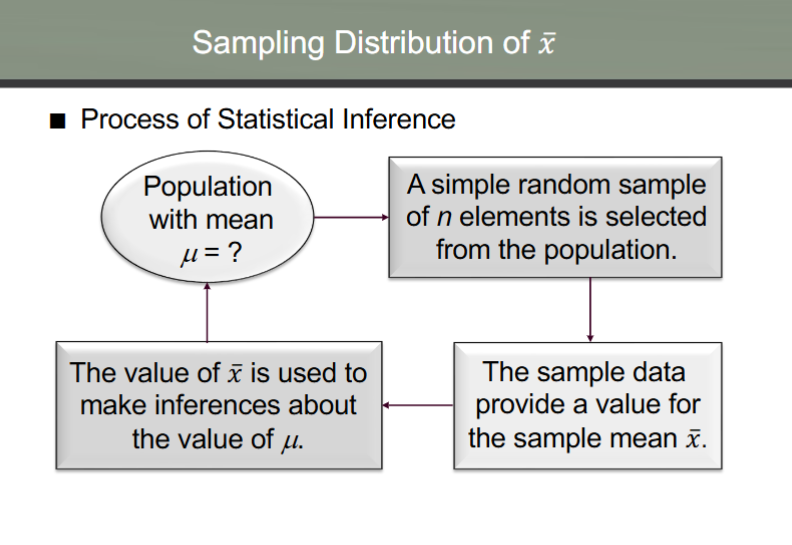
sampling distribution of x (sample mean)

• the probability distribution of all possible values of the sample mean

• expected value of sample mean = population mean

• when the expected value of the point estimator equals the population parameter, we say the point estimator is unbiased

sampling distribution of sample mean

• when the population has a normal distribution, the sampling distribution of x is normally distributed for any sample size

• in most applications, the sampling distribution of x can be approximated by a normal distribution whenever the sample is size 30 or more

• in cases where the population is highly skewed or outliers are present, samples of size 50 may be needed

• the sampling distribution of x can be used to provide probability info about how close the sample mean x is to the population mean u 

central limit theorem

• when the population from which we are selecting a random sample does not have a normal distribution, this theorem is helping in identifying the shape of the sampling distribution of x 

• in selecting random samples of size n from a population, the sampling distribution of the sample mean x can be approximated by a normal distribution as the sample size becomes large

other sampling methods

• stratified random sampling

• cluster sampling

• systematic sampling

• convenience sampling

• judgment sampling

stratified random sampling

• the population is first divided into groups of elements called strata

• each element in the population belongs to one and only one stratum

• best results are obtained when the elements within each stratum are as much alike as possible (ex: a homogeneous group)

• a simple random sample is taken from each stratum

• formulas are available for combining the stratum sample results into one population parameter estimate

• advantage: if strata are homogenous, this method is as “precise” as simple random sampling but w a smaller total sample size

• ex: the basis for forming the strata might be department, location, age, industry type, and so on

cluster sampling

• the population is first divided into separate groups of elements called clusters

• ideally each cluster is a representative small-scale version of the population (ex: heterogeneous group)

• a simple random sample of the clusters is taken

• all elements within each sampled (chosen) cluster form the sample

• ex: a primary application is area sampling, where clusters are city blocks or other well-defined areas

• advantage: the close proximity of elements can be cost effective (ex: many sample observations can be obtained in a short time)

• disadvantage: this method generally requires a larger total sample size than simple or stratified random sampling

systematic sampling

• if a sample size of n is desired from a population containing N elements, we might sample one element for every n/N elements in the population

• we randomly select one of the first n/N elements from the population list

• we then select every n/Nth element that follows in the population list

• this method has the properties of a simple random sample, especially if the list of the population elements is a random ordering

• advantage: the sample usually will be easier to identify than it would be if simple random sampling were used

• example: selecting every 100th listing in a telephone book after the first randomly selected listing

convenience sampling

• it is a nonprobability sampling technique. items are included in the sample w out known probabilities of being selected

• the sample is identified primarily by convenience

• ex: a professor conducting research might use student volunteers to constitute a sample

• advantage: sample selection and data collection are relatively easy

• disadvantage: it’s impossible to determine how representative of the population the sample is

judgment sampling

• the person most knowledgeable on the subject of the study selects elements of the population that he or she feels are most representative of the population

• it is a nonprobability sampling technique

• ex: a reporter might sample 3 or 4 senators, judging them as reflecting the general opinion of the senate

• advantage: it’s a relatively easy way of selecting a sample

• disadvantage: the quality of the sample results depends on the judgment of the person selecting the sample

recommendation

• it is recommended that probability sampling methods (simple random, stratified, cluster, or systematic) be used

• for these methods, formulas are available for evaluating the “goodness” of the sample results in terms of the closeness of the results to the population parameters being estimated

• an evaluation of the goodness cannot be made w non-probability (convenience or judgment) sampling methods

a point estimator cannot…

• be expected to provide the exact value of the population parameter

• an interval estimate can be computed by adding and subtracting a margin of error to the point estimate (point estimate ± margin or error)

• the purpose of an interval estimate is to provide info point how close the point estimate is to the value of the parameter

the general form of an interval estimate of a population mean is

sample mean ± margin of error

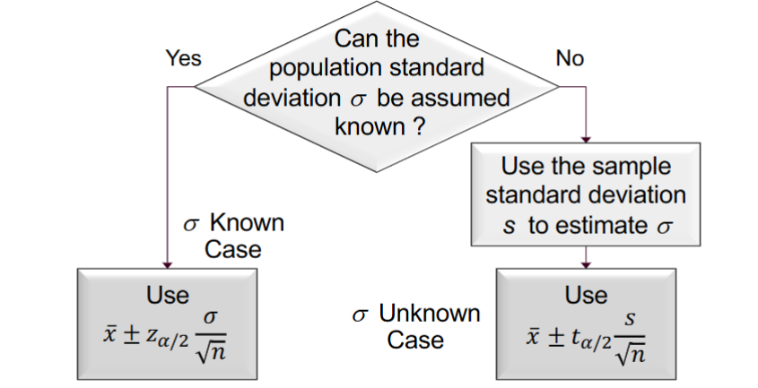
interval estimate of a population mean: sigma known

• in order to develop an interval estimate of a population mean, the margin of error must be computed using either:

  • the population standard deviation sigma, or

  • the sample standard deviation s

• sigma is rarely known exactly, but often a good estimate can be obtained based on historical data or other info

• we refer to such cases as the sigma known case

• there is a 1-a probability that the value of a sample mean will provide a margin of error or less

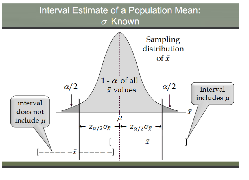
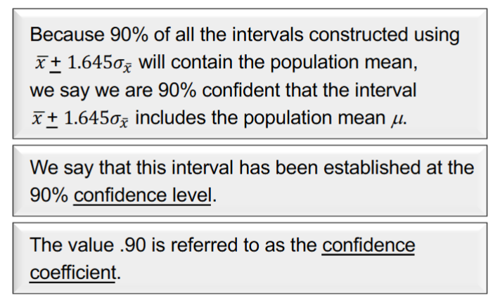
meaning of confidence

adequate sample size when sigma is known

• in most applications, a sample size of n=30 is adequate

• if the population distribution is highly skewed or contains outliers, a sample size of 50 or more is recommended

• if the population is not normally distributed but is roughly symmetric, a sample size as small of 15 will suffice

• if the population is believed to be at least approximately normal, a sample size of less than 15 can be used

interval estimate of a population mean: sigma unknown

• if an estimate of the population standard deviation sigma cannot be developed prior to sampling, we use the sample standard deviation s to estimate sigma

• this is the sigma unknown case

• in this case, the interval estimate for u is based on the t distribution

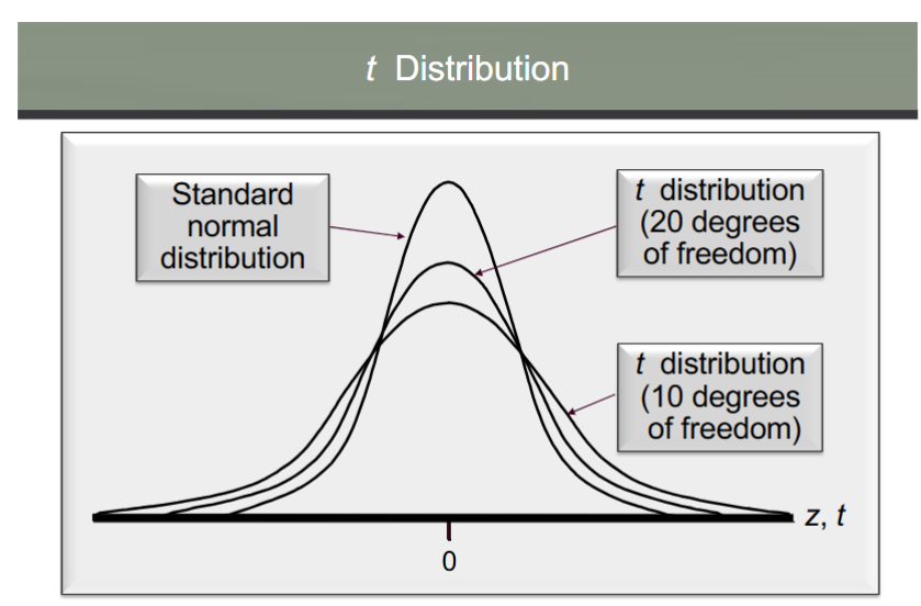
t distribution

• william gosset, writing under the name “student”, is the founder

  • oxford grad in math and worked for Guinness

  • developed it while working on small-scale materials and temperature experiments

• the t distribution is a family of similar probability distributions

• a specific t distribution depends on a parameter known as the degrees of freedom

• a t distribution w more degrees of freedom has less dispersion

• as df increases, the diff btw the t dist and the standard normal probability distribution becomes smaller and smaller

• for more than 100 degrees of freedom, the standard normal z value provides a good approximation to the t value

• the standard normal z values can be found in the infinite degrees row of the t distribution table

degrees of freedom

refer to the # of independent pieces of info that go into the computation of s

sigma unknown adequate sample size

• usually a sample size of n=30 is adequate to develop an interval estimate of a population mean

• if the population distribution is highly skewed or contains outliers, a sample size of 50 or more is recommended

• if the population is not normally dist but is roughly symmetric, a sample size as small as 15 will suffice

• if the population is believed to be at least approximately normal, a sample size of less than 15 can be used

summary of interval estimation procedures for a population mean

sample size for an interval estimate of a population mean

• let E = the desired margin of error

• E is the amount added to and subtracted from the point estimate to obtain an interval estimate

• if a desired margin of error is selected prior to sampling, the sample size necessary to satisfy the margin of error can be determined

planning value

• the Necessary Sample Size equation requires a value for the population st dev

• if sigma is known, a preliminary or planning value for sigma can be used in the equation

  • use the estimate of the population st dev computed in a previous study

  • use a pilot study to select a preliminary study and use the sample st dev from the study

  • use judgment or a best guess for the value of sigma