Factor markets

Marginal revenue product of labour

(Additional revenue generated from hiring one more unit of labour)

MRP_L = MP_L x MR

Under perfect competition in the goods market MR = P

so MRP_L = MP_L x P = VMP_L (Value of marginal product of labour)

Under imperfect competition MR < P

Marginal revenue product of labour - issue

From producer theory we know marginal product of labour declines with additional labour due to diminishing marginal returns, therefore marginal revenue product of labour ALSO decreases as more labour is hired

Under imperfect competition MR falls with output so MRP_L declines even faster

Inverse relationship between MRP_L and the quantity of labour hired.

Therefore for a firm they will hire labour up to the point when MRP_L = w

w = wage rate which represents the cost of hiring an additional unit of labour

Formula for optimal amount of labour employed

MRP_L = w

Or

MR = w/MP_L

Demand for labour

Derived demand as firms profit max output choice necessitates optimal labour hiring

Any factor that changes the MP_L or MR will shift the labour demand curve

The MP_L depends on the tech of the production process and the amount of capital employed

Effect of changes in wages

If there is no feedback from wages to output prices then a fall in wages only causes a movement along/down the labour demand curve - increasing quantity of labour demanded, but if there is feedback, the MR and demand for labour will shift inwards alongside the movement down the labour demand curve

Labour demand in the long run

In the short run capital is fixed so given a fall in wages the firm will hire more labour increasing productivity of labour, but in the long run the firm can adjust capital so will increase capital usage, and the demand for labour will be flatter (more elastic), due to increased responsiveness of labour demand to wages

Supply of labour - perfectly competitive market

Firm can hire any quantity at prevailing market wage, so wage is constant regardless of how much labour the firm demands/hires

Overall supply of labour depends on people’s willingness to work which varies with age, health, family responsibilities

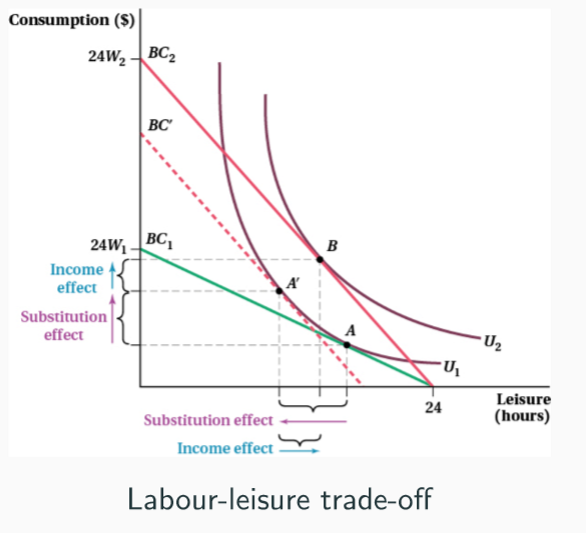
Labour leisure trade off

Leisure - normal good, but comes at a cost - the forgone income from not working

Labour - generates income which enables consumption so trade off between leisure and consumption

Decomposing the wage effect

A change in wage triggers the substitution and income effect

E.g. Increase in wage rate, means that the initial bundle of leisure and consumption chosen on the first indifference curve and budget line changes as the budget line pivots outwards, making leisure more expensive, and so there is a new bundle B on a new indifference curve and budget line

The substitution effect shows how the individual substitutes AWAY from leisure towards more work, as the budget line is shifted inwards so it crosses through the original indifference curve and the shift from A to A’ reflects this. Then the income effect shows how higher income (from higher wages) then increases demand for leisure, moving from A’ to B, so the total effect is shown by movement from A to B - on a higher indifference curve reflecting increased overall well-being.

The total effect depends on the relative strength/direction of the two effects and at lower wage levels the substitution effect dominates and vice versa

Monopsonist

A firm large enough that its hiring decision influence the market wage e.g. the NHS in the UK

As a large buyer of labour the firm faces an upward-sloping labour supply curve

The firm hires labour where its marginal expenditure (additional cost to hire one more unit of labour) = the marginal revenue product of labour

There is a dead weight loss which arises from underemployment of labour - workers willing to work at a higher wage but not hired even though their contribution exceeds the wage the firm would need to pay