22.11 Final Review

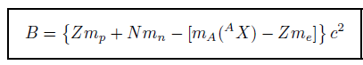
Binding Energy

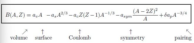
Semi-Empirical Mass Formula (SEMF)

Radius of a Nucleus Estimate

R~R0*A^1/3 where R0=1.25fm

SEMF Volume Term Reasoning

Because nucleons are closely packed and the nuclear force has a short range the Volume force is proportional to A (R³) instead of A*(1-A).

av

15.5 MeV

SEMF Surface Term Reasoning

Correction to the volume term since there are less nuclides to interact with on the surface of the nucleus. Proportional to A^(2/3) (R²)

as

13-18 MeV

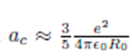
SEMF Coulomb Term Reasoning

Comes from the energy of a uniformly charged sphere ~Q²/R —> Q² = e²Z(Z-1)

ac

ac = 0.691

SEMF Symmetry Term Reasoning

Comes from the shell model of the nucleus and Pauli Exclusion Principle. IF you want to add more of one type of nucleon it must be more energetic which lowers the total binding energy. The (N-Z) term is squared because it better matches empirical data.

asym

23 MeV

SEMF Pairing Term Reasoning

Having even-even numbers of nucleons is the most energetically favorable configuration, while odd-odd is the least energetically favorable. Even-odd has no overall effect.

ap

34 MeV

How to find optimal numbers (N, Z, etc.) from the SEMF?

Differentiate with respect to the number of interest.

Q value

Difference in rest masses or kinetic energies

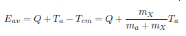
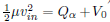
Center of Mass Kinetic Energy

Center of Mass Velocity

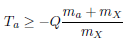
Available Energy

Reaction Condition

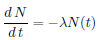
Radioactive Decay

Mean Lifetime

tau = 1/lambda

Half-life

t1/2 = ln(2)/lambda

Activity

A = lambda*N(t)

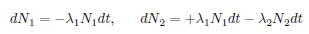
Chain of Decays

What nuclides is alpha decay observed for?

A > 200

Geiger-Nuttall Rule

log(t1/2) ~ 1/sqrt(Qalpha)

Beta Decay Parabolas

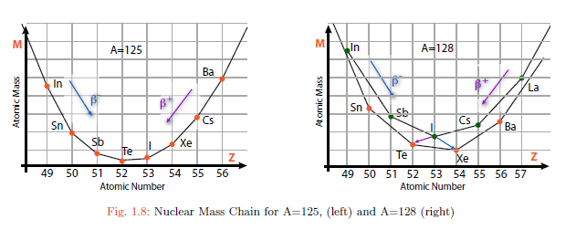
When doing Q-value equations for beta decay…

The mass of electrons matter

Gamma Energies

E = hbar*k*c = hbar * omega_k

Steps of a Quantum Mechanical Experiment

1. Preparation: determines the probabilities of the various possible outcomes (states)

2. Measurement: retrieve the value of a particular outcome, in a statistic manner (measurement of observables)

First Axiom of Quantum Mechanics

States: The properties of a quantum system are completely dened by specification of its state vector. The state vector is an element of a complex Hilbert space H called the space of states.

Second Axiom of Quantum Mechanics

Hermitian Operators: With every physical property (energy, position, momentum, angular momentum, ...) there exists an associated linear, Hermitian operator “A” (usually called observable), which acts in the space of states H. The eigenvalues of the operator are the possible values of the physical properties.

Third Axiom of Quantum Mechanics

a. Probability of States (Born Rule): The modulus squared of the inner product of two states gives the probability of finding one state in the other.

b. Probability of Operators and Wave Function Collapse: If A is an observable with eigenvalues a_n and eigenvectors |n>, the probability of obtaining a_n as the outcome of the measurement of A is p(a_n) = |<n|f>|². After the measurement, the system is left in the state projected on the subspace of the eigenvalue a_n.

Fourth Axiom of Quantum Mechanics

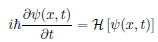
The evolution of a closed system is unitary (reversible). The evolution is given by the time-dependent Schrodinger equation.

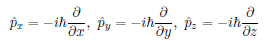
Momentum operator in position basis

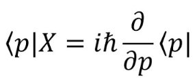
Position operator in momentum basis

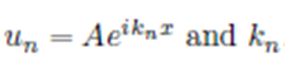
Momentum eigenfunctions and values

Kinetic energy wavenumber relation

Properties of eigenfunctions

1. The eigenfunctions of an operator are orthogonal functions

2. The set of eigenfunctions forms a complete basis (any other vector functions belonging to the same space can be written in terms of the set)

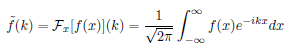
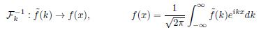
Fourier Transform

Inverse Fourier Transform

Procedure for calculating all of the probabilities of each outcome for each observable

1. Find the eigenfunctions of the observable’s operator

2. Find the probability amplitude of the wavefunction with respect to the eigenfunction of the desired eigen-value outcome

3. The probability of obtaining the given eigenvalue in the measurement is the probability amplitude modulus square

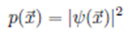
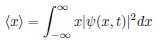
Position probability function

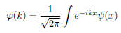
Momentum eigenfunctions…

cannot be normalized, they are a Fourier Transform of the position eigenfunction

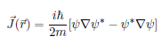
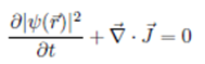
Probability flux

Conservation Equation

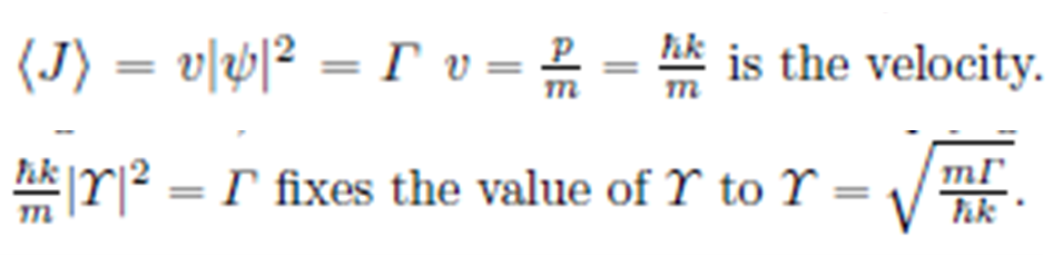
Free particle flux

Wavefunction expectation value

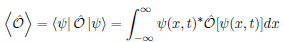
Operator Expectation Value

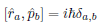
Position and Momentum Commutator

Commutator Properties

1. Any commutator commutes with scalars [A, a] = 0

2. [A, BC] = [A,B]C + B[A,C] and [AB,C] = A[B,C] + [A,C]B

3. Any operator commutes with itself [A,A] = 0 and with any power or functions of itself

Energy eigenfunctions are also…

momentum eigenfunctions

Eigenvalue degeneracy

Energy eigenfunctions are degenerate, there are two eigenfunctions associated with the same eigenvalue. The degeneracy is broken by measuring the momentum eigenvalue.

Complete Set of Commuting Observables

A set of operators that completely define the state. The eigenvalues are called good quantum numbers.

Time Dependent Schrodinger Equation

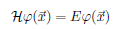
Time Independent Schrodinger Equation

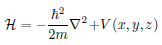
Position representation Hamiltonian

Total wavefunction

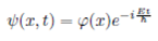
General solution of Schrodinger equation

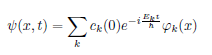
Energy eigenfunctions

Finite Potential Wall Boundary Conditions

YI(0) = YII(0) Y’I(0) = Y’II(0)

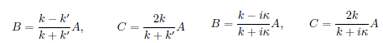
Finite Potential Wall Coefficients E>V and E<V

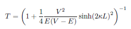
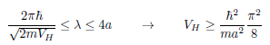
Tunneling probability

The initial energy in an alpha decay is equal to

the Q value of the reaction

Size of alpha decay potential well

R = R’ + R_alpha = R_0*((A-4)^1/3 + 4^1/3)

Alpha coulomb potential height

Alpha decay rate

(Probability of tunneling) x (Frequency at which the initial nuclei and alpha particle are found separately)

Alpha separation frequency

f = v_in/R = (velocity of particles in the nucleus)/(Potential well radius)

v_in

R_C

Solve for Q_alpha = V_C

Alpha decay rate

Gamow factor (approx)

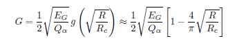
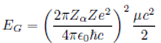
Gamow energy

Why are alpha decay more likely than spontaneous fission?

The Coulomb barrier becomes too large for other types of decay even though the Q-value is much larger

Infinite well boundary conditions

YI(0) = YII(0) (no derivative)

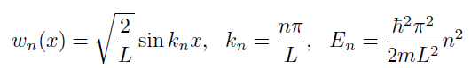
Infinite well wavenumber values

k_n = n*pi/L

Infinite well eigenfunction

Finite well odd solution constraints

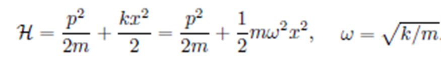
Harmonic oscillator Hamiltonian

Annihilation and creation operators

a|n> = sqrt(n)|n-1> a*|n> = sqrt(n+1)|n+1>

Number operator

N = a*a

Spherical coordinates

x = r*sin(t)*cos(p)
y = r*sin(t)*sin(p)
z = r*cos(t)

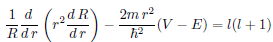
3D SE Radial

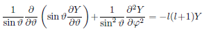
3D SE Angular

Angular Momentum Commutators

[Li, Lj] = i*hbar*Lk

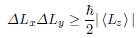
Angular momentum uncertainty relation

L² eigenvalue

L² |l,m> = hbar²l(l+1)|l,m>

Lz eigenvalue

Lz|l,m> = m*hbar|l,m>

Range of m values

-l, -l + 1, …, l - 1, l

<L²> in terms of Lz, Ly, and Lx

<L²> = <L²x> + <L²y> + <L²z>

Uncoupled representation

|l1, m1, l2, m2>

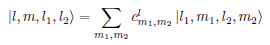
Coupled representation

|l, m, l1, l2>

Uncoupled representation to coupled representation

Angular momentum degeneracy

D = 2*l + 1

Total angular momentum bounds

|l1 - l2| < l < l1 + l2

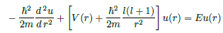
u(r) SE equation

3D Potential well effective potential

V(r) + centrifugal potential

Fermions

Particles with half-integer spin that cannot occupy identical states

Bosons

Particles with integer spin that can occupy identical states

Particles subject to the nuclear force

Protons and neutrons