Applied econometrics lecture 16 Differences in differences

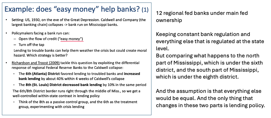
Bank run example overview

Assumption is that everything else would be equal

Only thing that changes in these two parts is lending policy

Therefore can compare effects of treatment (8th as control & 6th as treatment - crisis lending)

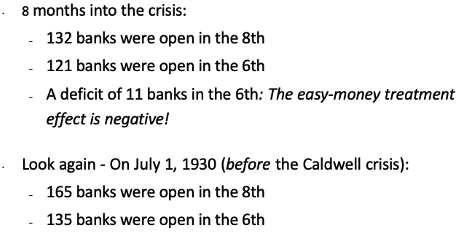
8 months into crisis

More banks open in 8th than 6th

However more were open in 8th to begin with

we have to use Difference in difference to adjust for this

DD additive model

The heart of the DD setup is an additive model for potential outcomes in the no-treatment state:

• Y_d,t (0) = β_d + γ_t

Y_d,t (0)

the potential outcome describing what happens in district d and period t in the absence of an intervention

β_d

District effect

• Certain districts on average have more or fewer banks

Time-invariatnt

γ_t

Year effect

• something at national level affecting no. banks

Common period

DD for banks

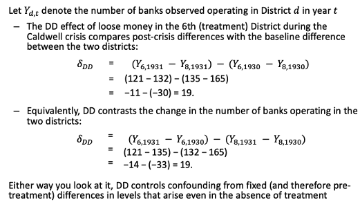
Treatment effect with DD

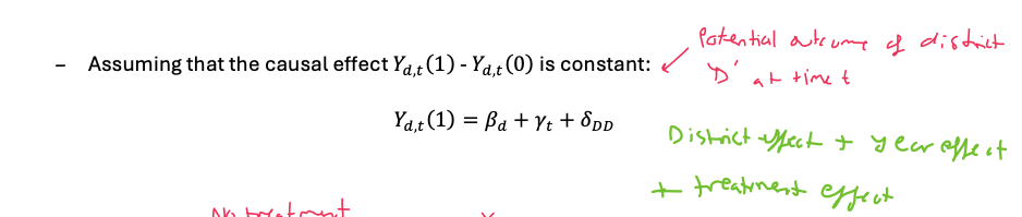
δ_DD - treatment effect

δ_DD

Treatment effect

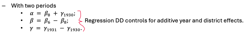
Treatment effect on banks - maths

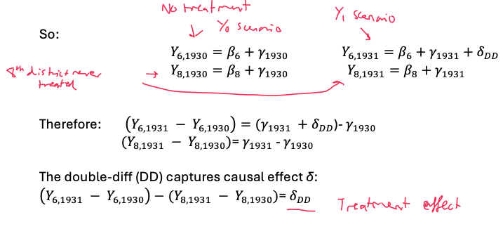
β drop out as same district in both years

γ drops out when comparing both districts as same year

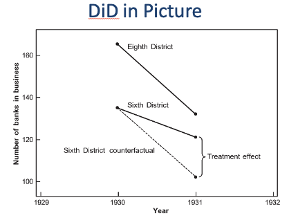
DD banks treatment effect - graph

We assume that treated would evolve like untreated if no treatment - counterfactual

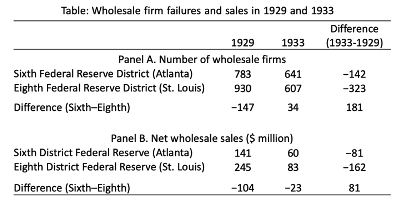
DD and causal effect - banks

Difference = 181 (no. of wholesale firms)

Difference = 81 (no. of wholesale sales)

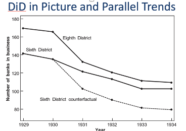
DD assumption - parallel outcome trends

Assume to generate counterfactual

Cant be tested in reality

But we can test whether the outcome evolves in parallel in periods that are not treated

– Pre-trends testing

– Both treated or both untreated

DD extendin time periods

time period extended to compare pre and post treatment

Regression to test counterfactual

TREAT_d - dummy for district effects (1 if 6th)

POST_t - dummy for post treatment years (1 if post)

δ_rDD - coefficient on interaction term of POST and TREAT to isolate treatment effects (regression treatment effects)

δ_DD vs δ_rDD

With 2 periods they coincide (are equal)

With more periods δ_rDD is more precise than simple 4 number equation

• rDD allows for fact that additive model fits imperfectly

δ_rDD

Regression treatment effect

–      generates SEs (but beware of serial correlation)

–      facilitates specification testing

–      Can add controls

Min wage Krueger DiD example overview

in 1992 New Jersey raised its minimum wage from $4.25 to $5.05

They use a DiD comparing change in employment in fast food restaurants in NJ to that in neighboring Pennsylvania , where the Min wage was flat at $4.25

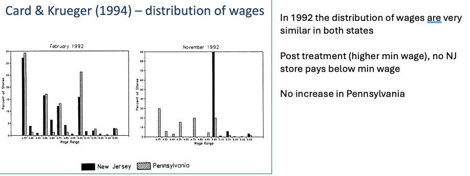
Min wage Krueger DiD example graph

Pre treatment - both states very similar distribution of wages

Post treatment - NJ has higher min wage + no increase in PA

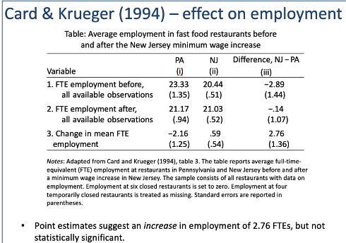
Min wage Krueger DiD example econometrics

Min wage increased employment → against standard theory

• statistically insignificant

Evolution before and after arent parallel + only 2 states used

Min wage Krueger DiD example findings explained

L market no perfectly competitive

• monopsonistic

Hiring new woker brings profit but w increases

• increases costs a lot

if Min w introduced then w has to rise anyway so firm hires more

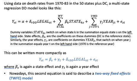
Two way fixed effects model (TWFE)

Extends regression to include 50 states & 13 years (not just 2 like before)

Regression compacted to look like additive model from before → from LSD (when all dummies shown)

Clustered standard errors

Clustered standard errors extend the OLS variance formula to allow (Y_it , X_it) to be correlated across observations in the same “cluster”

The assumption is that each cluster is sampled independently

If we cluster at the individual level (i), then we allow for Y_i1 and Y_i2 to be dependent, but assume (Y_i1, Y_i2) is independent of (Y_j1, Y_j2) for j ≠ iC

Clustered standard errors and panel data

At minimum cluster at the individual level to allow for autocorrelation.

Are clustered standard errors reliable when small?

No

<20

the number of “effective observations” (used for CLT) is the number of clusters

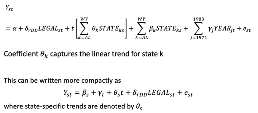
Relaxing the common trends assumption

With many states (β) and years (γ) we can relax the common trend assumption

We allow for seperate linear trends for each state (θ_k)

Regression with state specific trends

Ideal parallel trends scenario

Effect of treatment very visible

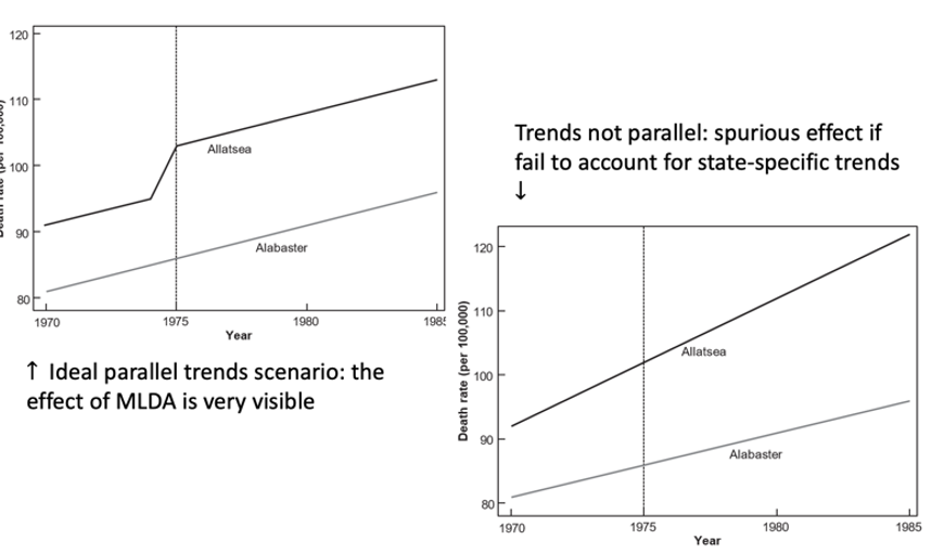
Effect of (minimum legal drinking age) MLDA very visible

Non parallel trends scenario

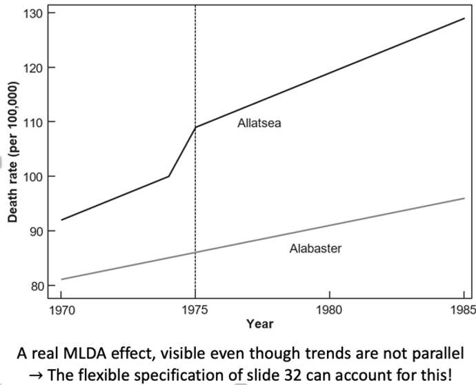
Dynamic treatment effect