FRM Part 4 Valuation and Risk Models

A key limitation of Value-at-Risk (VaR) that makes it not a coherent risk measure is that it:

It is not subadditive. Subadditivity would require that the risk measure of a combined portfolio should not exceed the sum of the risk measures of the individual portfolios, which VaR does not always satisfy.

According to Artzner’s definition, a coherent risk measure must satisfy monotonicity, subadditivity, positive homogeneity, and translation invariance. Describe how VaR violates subadditivity:

VaR can violate subadditivity (the VaR of a combined portfolio can exceed the sum of the VaRs of its components, especially with fat tails or concentrated positions). This property failure is why Expected Shortfall (ES) is preferred as a coherent alternative.

Consider two investment portfolios, Portfolio P and Portfolio Q. Due to their structuring with complex derivatives, it has been mathematically proven that in every possible future market state, the loss from Portfolio P is guaranteed to be greater than or equal to the loss from Portfolio Q. No scenario exists where Q loses more than P.

According to the properties of a coherent risk measure, what must be the relationship between the risk measures of Portfolio P and Portfolio Q?

The risk measure of P must be greater than or equal to the risk measure of Q - this scenario describes the monotonicity test. This states that if a portfolio always produces a worse result (in this case, a greater or equal loss) than another portfolio, its risk measure should reflect that by being greater than or equal to the risk measure of the superior portfolio.

An analyst is examining the diversification benefits of combining two risky assets, Asset X and Asset Y. She plots the set of all possible risk-return combinations for portfolios of X and Y under different assumptions for the correlation coefficient () between their returns.

How does the curvature of the efficient frontier for this two-asset portfolio change as the correlation coefficient () decreases from +1.0 toward -1.0?

The frontier becomes more curved, shifting further to the left.

The degree of curvature in a two-asset efficient frontier is a direct visual representation of the diversification benefit. When two assets are perfectly correlated (ρ=1.0), there is no diversification benefit; combining them simply results in a portfolio with a risk-return profile that is a linear combination of the two, forming a straight line. As the correlation decreases, the returns of the assets move less in tandem, allowing for a reduction in portfolio risk that is greater than the linear combination. This benefit appears as a curve, or bow, to the left in risk-return space. The lower the correlation, the more pronounced the curve, with the maximum curvature (and thus maximum diversification benefit) occurring at perfect negative correlation (ρ=−1.0).

Spectral risk measures provide a flexible framework for creating coherent risk measures tailored to specific risk preferences. Both VaR and ES can be viewed within this framework, with VaR having an incoherent weighting scheme and ES having the simplest coherent one. Describe how risk aversion can be built into this:

The risk aversion profile is embedded in the "spectrum," which is the function that defines the weights. An investor who is risk-neutral about tail losses would use ES (equal weighting). An investor who is extremely risk-averse to tail losses would use a function that assigns rapidly increasing weights to the tail.

A team of quantitative analysts is developing a new internal risk measure and must ensure it is coherent. They are testing the property of homogeneity. They begin with a base portfolio and calculate its risk measure. They then create a second portfolio by exactly doubling the position size of every asset in the base portfolio, with no change in market conditions or liquidity.

According to the homogeneity property of a coherent risk measure, what should be the relationship between the risk measure of the new, larger portfolio and the original portfolio?

The new risk measure should be exactly double the original risk measure.

The homogeneity property of a coherent risk measure states that changing the size of a portfolio by multiplying the amounts of all its components by a factor λ should result in the risk measure being multiplied by the same factor λ. In this scenario, the portfolio size is doubled (λ=2). Therefore, a coherent risk measure must also double. This property reflects the intuitive idea that if you double your bets, you double your risk, assuming no other changes like market liquidity impact.

The typical distribution of financial asset returns is not normal. How can the shape of the distribution be described?

Leptokurtic, meaning it is more peaked around the mean and has "fatter tails" i.e has positive excess kurtosis (kurtosis greater than 3).

The peakedness means that small changes (returns close to the mean) happen more often than a normal distribution would suggest. The fatter tails mean that large changes or extreme events (both gains and losses) also happen much more often than predicted by the normal distribution. Consequently, intermediate-sized moves happen less often.

A portfolio manager operates within the mean-variance framework, having constructed an efficient frontier using only risky assets. Upon introducing a risk-free asset available for both borrowing and lending at a single rate, the investment opportunity set is fundamentally reshaped. The manager must now advise a diverse client base, ranging from extremely risk-averse to highly risk-seeking investors.

How does the introduction of this risk-free asset alter the composition of the optimal portfolio of risky assets for all investors, regardless of their individual risk tolerance?

All investors hold the same portfolio of risky assets tangent to the new frontier.

When we introduce a risk-free asset that allows for both borrowing and lending, we create a new, linear efficient frontier. This new line is tangent to the original curved frontier of risky assets, and that single point of tangency represents what we call the 'market portfolio'—the one optimal portfolio of risky assets. The critical insight here is that every investor, no matter their tolerance for risk, should hold this same market portfolio. They then tailor their overall risk exposure by allocating funds between this market portfolio and the risk-free asset. A conservative investor will lend at the risk-free rate (buy the risk-free asset), while an aggressive investor will borrow at that rate to leverage their position in the market portfolio. The composition of the risky part of their holdings remains identical.

The Capital Asset Pricing Model (CAPM) builds directly on the mean-variance framework and the efficient frontier. The line extending from the risk-free rate through the market portfolio is known as the Capital Market Line (CML). What are some assumptions around this?

• This conclusion that all investors hold the same market portfolio relies on several strong assumptions, including that all investors have the same expectations about returns, standard deviations, and correlations, and can borrow and lend at the same risk-free rate.

• In practice, investors have different views and constraints, leading them to hold different risky portfolios. However, the model provides a powerful theoretical benchmark for portfolio construction.

• The "market portfolio" theoretically includes all available risky assets in the market, weighted by their market capitalization.

VaR provides an estimate of the minimum loss that could occur with a certain probability, not an exact loss amount.

What does the statement “due to volatility in oil prices, the company has a weekly 90% VaR of €20,000” mean?

A 90% VaR of €20,000 means that there is a 10% chance that losses will exceed €20,000 in any given week.

The losses from a portfolio for one year are normally distributed with mean -10 and standard deviation 20. What is the value of the 99% expected shortfall?

42.85

For a confidence level of 99%, we find the z-score by inverting the cumulative distribution function (CDF), Φ−1, of the standard normal distribution:

U=Φ−1(0.99)=2.33

This z-score represents the point at which 99% of the distribution's values fall below it.

With our z-score U and the known values for the mean μ=−10 and standard deviation σ=20, we can now plug these into the ES formula:

ES=−10+20⎛⎝⎜e−2.332/2/(1−0.99)2π−−√⎞⎠⎟=42.85

This means that, at the 99% confidence level, the expected shortfall of the portfolio—the average loss in the worst 1% of cases—is approximately $42.85 million

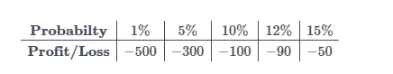
An investment company has a portfolio which has the following ordered performance by historical data. Calculate the expected shortfall ES0.95.

To calculate the expected shortfall, we must ask ourselves, "If we are in the worst 5% of the loss distribution, what is the expected loss?" The first column of the given table makes it clear that the 5% tail of the distribution is composed of a 1% probability that the loss is 500 and a 4% probability that the loss is 300. Conditional on being in the tail of the distribution, there is, therefore, a 1/5 chance that the loss is 500 million and a 4/5 chance that it is 300. The expected shortfall (in millions of dollars) is, therefore:

(1/5)×500+(4/5)×300=340

A financial analyst uses the delta-normal approach to calculate the 1-day VaR of a portfolio composed of non-linear derivatives like options. The portfolio's delta is 0.5, the underlying's price volatility is 20%, and the initial value of the underlying is $100. Assuming a 95% confidence level, what is the 1-day VaR of this portfolio?

To compute the 1-day Value at Risk (VaR) using the delta-normal approach, we use the following formula:

VaR=|Δ|⋅S⋅σ⋅z⋅√Δt

Where:

• Δ=0.5 (portfolio delta)

• S=100 (underlying price)

• σ=0.20 (volatility)

• z=1.645 (Z-score for 95% confidence level)

• Δt=1 (1-day horizon)

Substituting the values:

VaR=0.5⋅100⋅0.20⋅1.645=16.45

Therefore, the 1-day VaR at 95% confidence is $16.45

Define Delta in the context of options:

Delta represents the rate of change of an option's or portfolio's value with respect to changes in the price of the underlying asset. It measures the sensitivity of the option's value to small movements in the underlying asset's price.

Delta is a first-order risk measure, indicating the linear sensitivity of the portfolio's value. For example, a delta of 0.5 means that for every $1 increase in the underlying asset's price, the option's value will increase by $0.50.

Why might the delta-normal approach underestimate the risk for portfolios with significant non-linear derivative positions?

It inadequately models the higher-order risks associated with non-linear derivatives. The delta-normal approach may underestimate risk for significant non-linear derivatives because it inadequately models higher-order risks like gamma and vega, which are crucial for capturing the curvature and volatility sensitivity in derivatives’ values.

A risk manager is evaluating the effectiveness of different risk measures for a portfolio that includes equities, bonds, and derivatives. The manager wants to ensure that the chosen risk measure can adequately handle non-linear instruments and capture extreme market movements. Which of the following risk measures would be most appropriate in this scenario?

Monte Carlo VaR is particularly effective for portfolios that include non-linear instruments like derivatives and for capturing extreme market movements. The method uses simulations to model a wide range of possible outcomes, allowing it to handle the complexities and non-linearities inherent in such portfolios.

A notable weakness of the Monte Carlo simulation method is its sensitivity to input assumptions and the extensive computational resources required. The accuracy of the output depends strongly on the quality of the input assumptions, and simulations can be time-consuming and resource-intensive.

During the 2007-2008 financial crisis, many financial institutions observed a significant change in the correlations between asset returns under stressed market conditions. What is this phenomenon known as, and what implication does it have for VaR or ES analysis?

This phenomenon is known as correlation breakdown. During stressed market conditions, asset return correlations often increase. This implies that standard risk models, which typically assume stable correlations, may underestimate risk during stress periods, making VaR and ES calculations less reliable. Adjustments for time-varying correlations are necessary to improve risk estimation accuracy under stress scenarios. i.e a financial institution should incorporate stressed correlations estimated from historical periods of high volatility.

Correlation breakdown reduces diversification benefits, making traditional VaR and ES models underestimate risk during market stress. i.e overestimate diversification and underestimate potential losses.

How does correlation breakdown impact ES models?

Correlation breakdown, where correlations between assets increase significantly during market stress (e.g., all assets decline together), causes ES analysis to underestimate potential losses if the model assumes stable or lower correlations. ES, which measures the average loss in the tail, is particularly sensitive to correlated losses, amplifying tail risk

Linear portfolios are well-suited to simpler risk models like the delta-normal approach, while non-linear portfolios often require more complex methods like Monte Carlo simulation. What ae some examples of non-linear products?

Non-Linear Portfolios: Contain instruments like options or mortgage-backed securities. Their risk profile includes curvature (gamma), which means linear approximations can be highly inaccurate, especially for large market moves.

In the historical simulation approach, it's standard practice to treat different types of risk factors differently. How should stock prices, FX and interest rates be modelled?

For market variables like stock prices and exchange rates, which tend to exhibit growth over time and are unbounded, it's more appropriate to model their percentage changes. This approach assumes that historical percentage moves are a better guide to future percentage moves.

For variables like interest rates and credit spreads, which are typically range-bound and quoted in specific units (percent or basis points), it is standard to model their actual changes.

The delta-normal model (aka variance-covariance approach) gets its name from its two core assumptions. What are these?

1) First it assumes that the change in the portfolio's value is a linear function of the changes in its underlying risk factors, an approximation captured by delta.

2) Second, it assumes that the changes in the risk factors themselves follow a multivariate normal distribution. These two assumptions together imply that the change in the portfolio's value will also be normally distributed, which makes calculating VaR a straightforward statistical exercise based on the portfolio's mean and standard deviation. The model's reliance on the normality assumption is a major weakness, as financial returns are known to have "fat tails."