Chapter 22: Cost Curves

cost curve

the graph of a cost function; a mathematical relationship between a firm's production costs and its output

What is the mathematical notation for variable costs associated with a given output, y, in economics?

cv(y)

How can the total costs that a firm incurrs be written mathematically in terms of fixed costs and variable costs?

c(y) = cv(y) + F

• c(y): total costs for a given output, y

• y: a given level of output

• cv(y): variable costs associated with a given output, y

• F: fixed costs

Average Cost Function (AC)

function that measures the cost per unit of output

Average costs are composed of average variable costs plus average fixed costs. Average fixed costs always decline with output, while average variable costs tend to increase. The net result is a U-shaped average cost curve.

• Increasing returns to scale implies decreasing average cost

• decreasing returns to scale implies increasing average cost

• constant returns to scale implies constant average cost

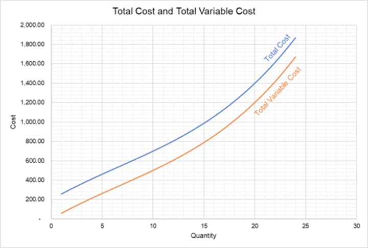
average variable cost function

a function that measures the variable costs per unit of output

• Notation: AVC(y)

average fixed cost function

a function that measures the fixed costs per unit output

• Notation: AFC(y)

Construction of the average cost curve

• It's beneficial for a business to make as many units of output as possible when faced with a fixed cost, since fixed costs are allocated with each unit of output.

• EX: Say it costs a farmer a flat fee to use a truck load to ship strawberries. It would make sense for the farmer to put as many strawberries as possible in the truck to reduce the true cost of using that truck load (the expense is allocated over the units, so maximizing units will reduce per unit cost).

• Variable costs make the average cost of producing a given good increase as more products are produced

• Costs that have both a fixed element and a variable element will have a "U" shaped cost curve because eventually the variable element of the costs will overwhelm the fixed element.

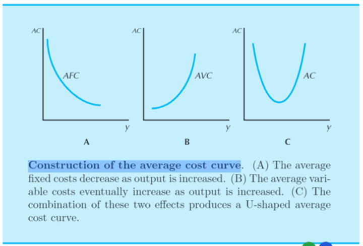
average cost curve

a "u-shaped" graph that conveys both the variable and fixed costs of producing a given level of output

• the "U-shape" is due to initial decline in average costs, which in turn is due to the decline in average fixed costs

• the eventual increase in average costs is due to the increase in average variable costs

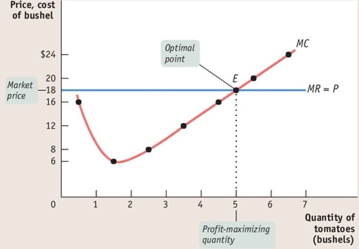
marginal cost (MC) curve

a graph that describes how the cost of producing one more unit depends on the quantity that has already been produced

• Calculus: Difference Quotient = MC(y)

= ( c(y +Δy) - c(y) ) / Δy

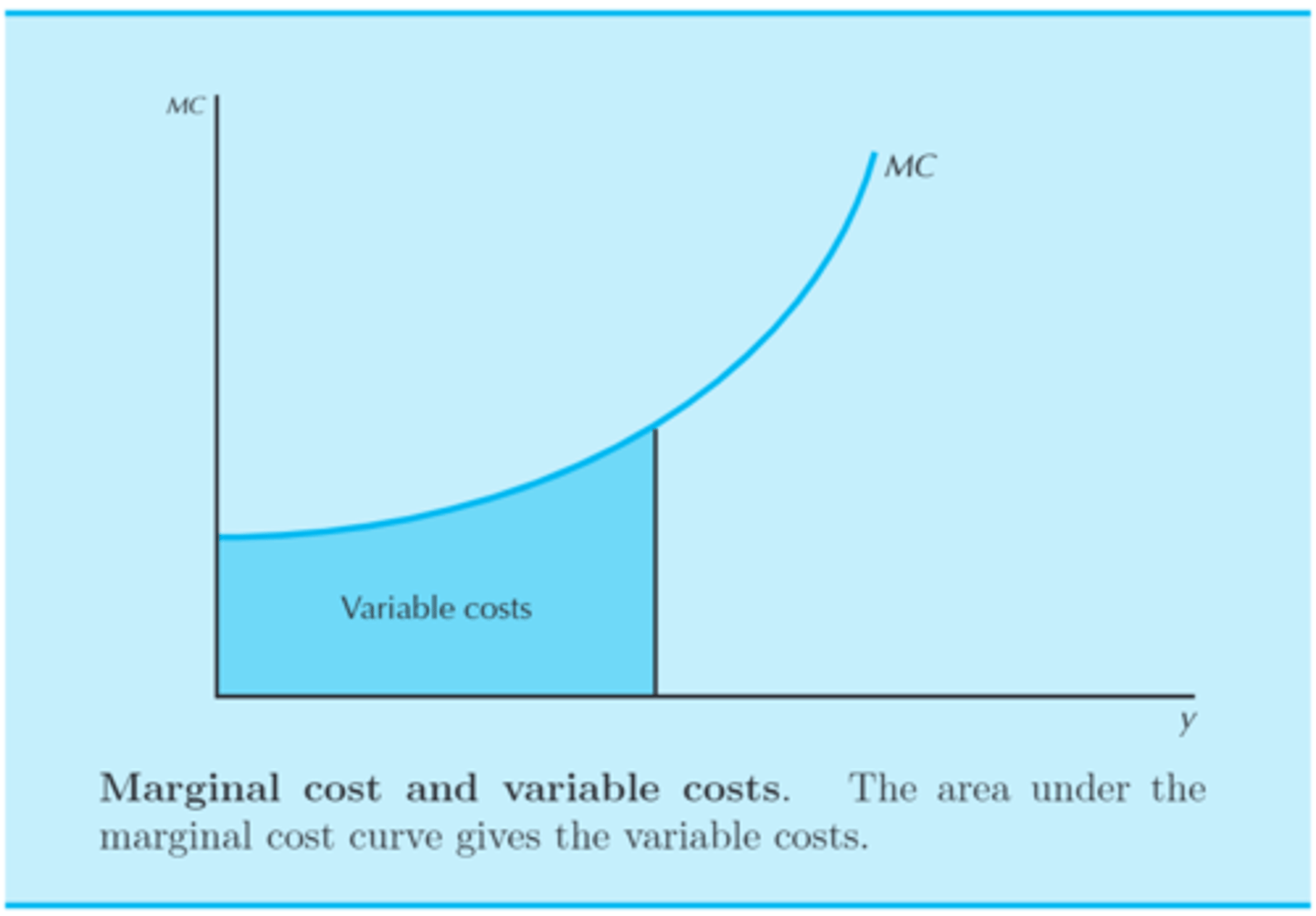
• The area under the marginal cost curve describes the variable costs.

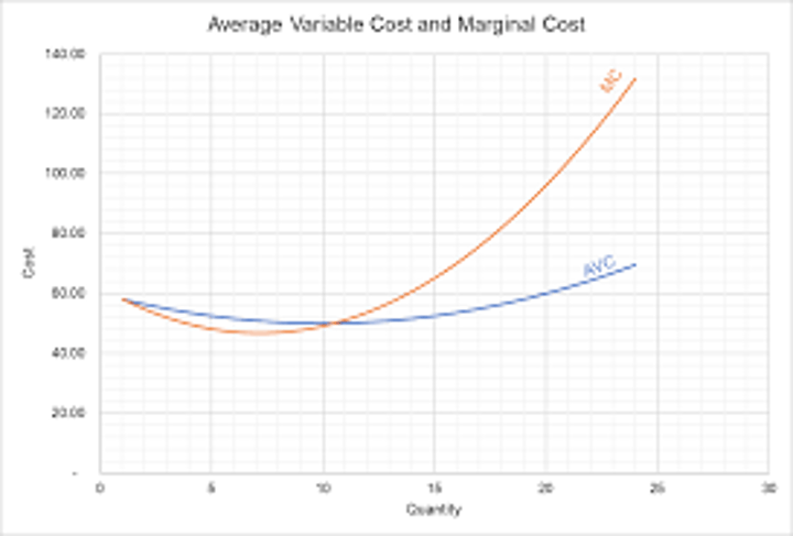
• The marginal cost curve lies below the average cost curve when average costs are decreasing, and above when they are increasing. Thus marginal costs must equal average costs at the point of minimum average costs.

What does the marginal cost measure?

Marginal cost measures the change in costs divided by a change in output

Marginal Cost (MC)

the change in total costs associated with a one-unit change in output

What can be inferred about the marginal costs of a good if its average variable costs are decreasing?

It must be that the marginal costs are less than the average variable costs in this range.

WHY?

If the average is decreasing, it must be that the cost of each additional unit produced is less than average up to that point.

• Similarly, if we are in a region where average variable costs are rising, then it must be the case that the marginal costs are greater than the average variable costs— it's the higher marginal costs that are pushing the average up.

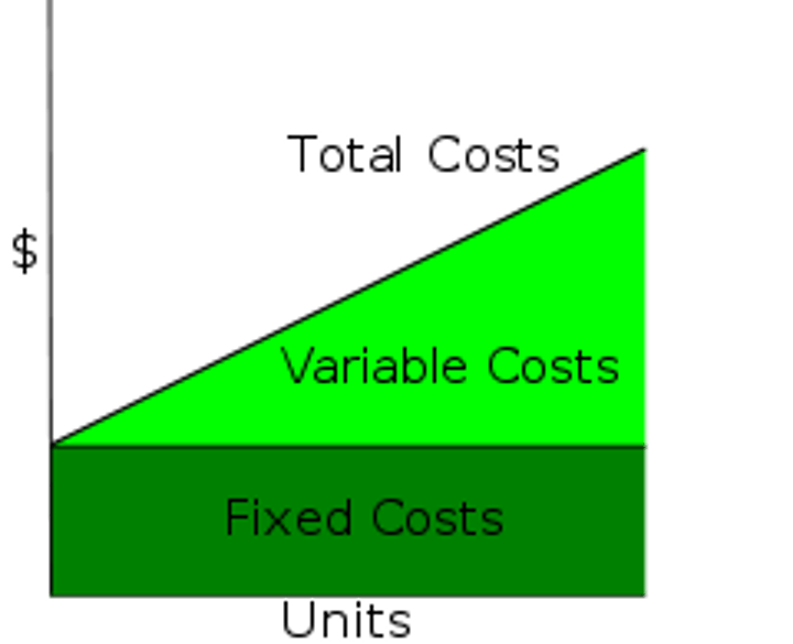
variable costs

costs that vary with the quantity of output produced

• EX: fuel expenses of an airline company

fixed costs

costs that remain constant regardless of the amount of output produced

• bill for lighting in a facility

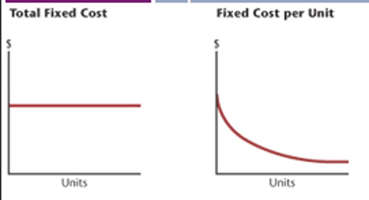
The average cost curve will initially fall due to declining _____ costs but then rise due to the increasing average ________ costs.

The average cost curve will initially fall due to declining fixed costs but then rise due to the increasing average variable costs.

What is the difference in value between the marginal cost and average variable cost if only one unit of output has been produced?

None-- they are both exactly the same value if only one output has been produced.

The marginal cost curve passes through the ________ point of both the average variable cost and the average cost curves.

The marginal cost curve passes through the minimum point of both the average variable cost and the average cost curves.

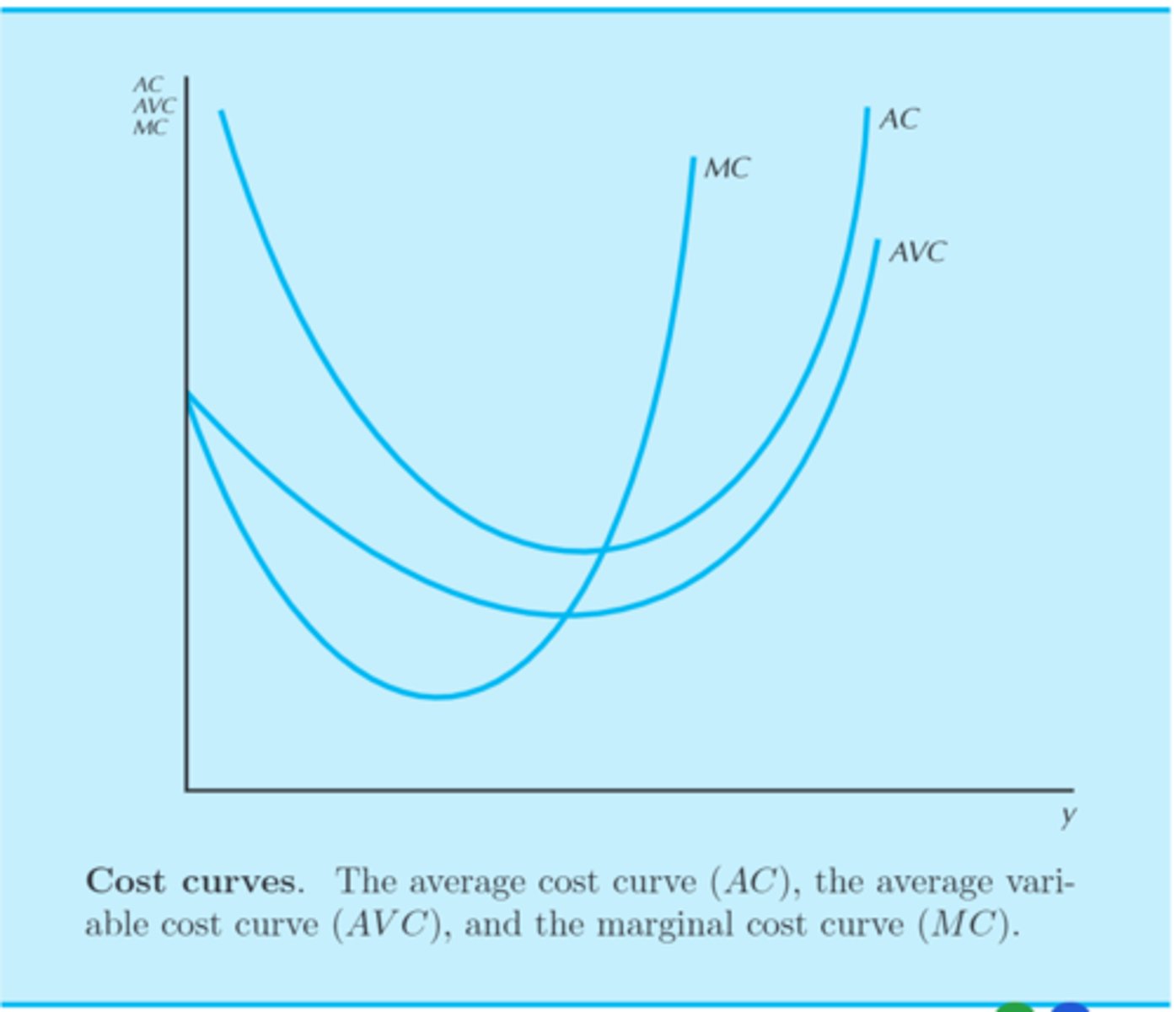
The area under the marginal cost curve describes the ________ _______.

variable costs

• see diagram

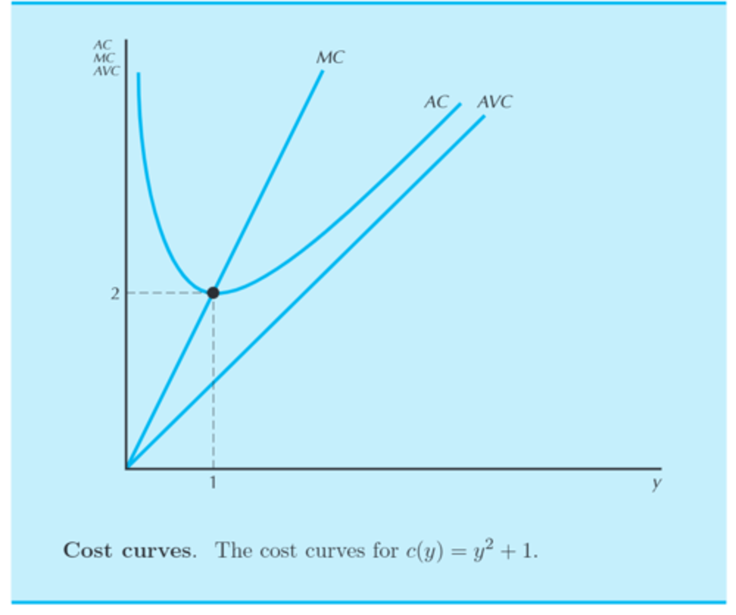
Consider the cost funtion c(y) = y^2 + 1 , where "y" is number of output produced.

What are the following derriced cost curves?

A) variable costs
B) fixed costs
C) Average variable costs
D) average fixed costs
E) average costs
F) Marginal costs

A) cv(y) = y^2

B) cf(y) = 1

C) AVC(y) = y^2/y = y

D) AFC(y) = 1/y

E) AC(y) = (y^2 + 1) / y = y + (1/y)

F) MC(y) = 2y

• Note that the Marginal Costs function is the derivative of the corresponding cost function (Study Calculus if you don't know how to find a derivative).

What is the derivative of c(y) = y^2 + F

• F is a constant

The derivative is "2y".

• Study basic calculus if you don't know how this is found.
• For economics, you can memorize this fact even if you don't know calculus to find the marginal product of simple cost functions.

The average cost curve reaches its minimum when the average cost equals the _______ _____.

marginal cost

EXAMPLE

If the cost function is "c(y) = y^2 + 1", then the average cost is "y + (1 / y)" and the marginal cost is "2y".

• Therefore, the minimum is when "y + (1 / y) = 2y"

• Solving for y: y = 1

According to the cost funtion, if y is "1", then the average cost will be "2". Therefore, In this example, the minimum cost occurs when one unit is produced. And the associated cost for producing one unit is $2.

• see diagram for the example being graphed

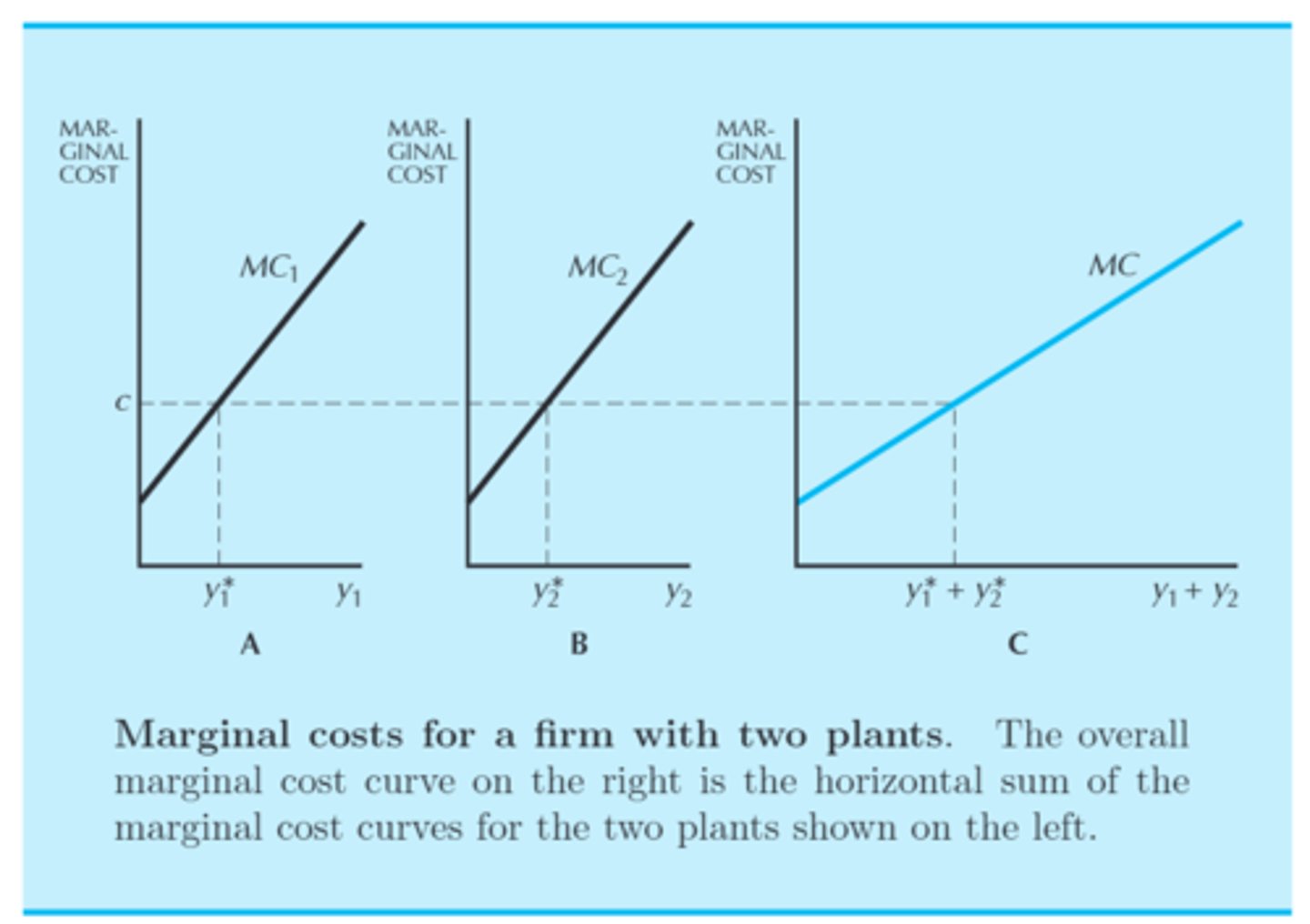
Suppose there are two factories, and an entrepreneur wants to produce a certain number of goods (y) as cheaply as possible. That entrepreneur would have to figure out how much of each output should be produced from each factory.

What is a mathematical expression that would solve this problem?

min of y', y": c'(y') + c"(y")

such that y' +y" = y

• Each cost function, c(y), corresponds to the two factories.

"Min." is used to denote that the cheapest method is desired

• y': output of factory #1; y": output of factory #2

• y: total output

The marginal cost of producing output at factory #1 must be equal to the marginal cost of producing output at factory #2 to find how much output should be produced from each factory to find the cheapest way to produce a specified total output. That value would also be the horizontal sum of the marginal cost curves.

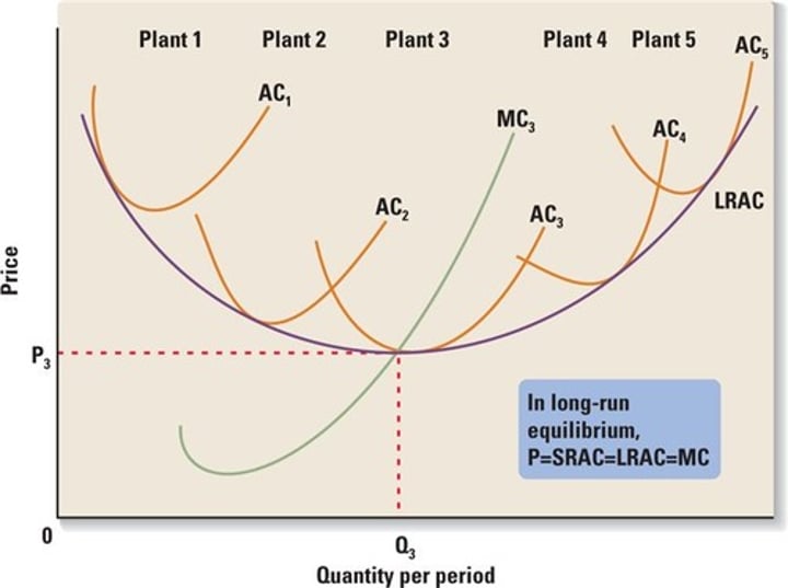
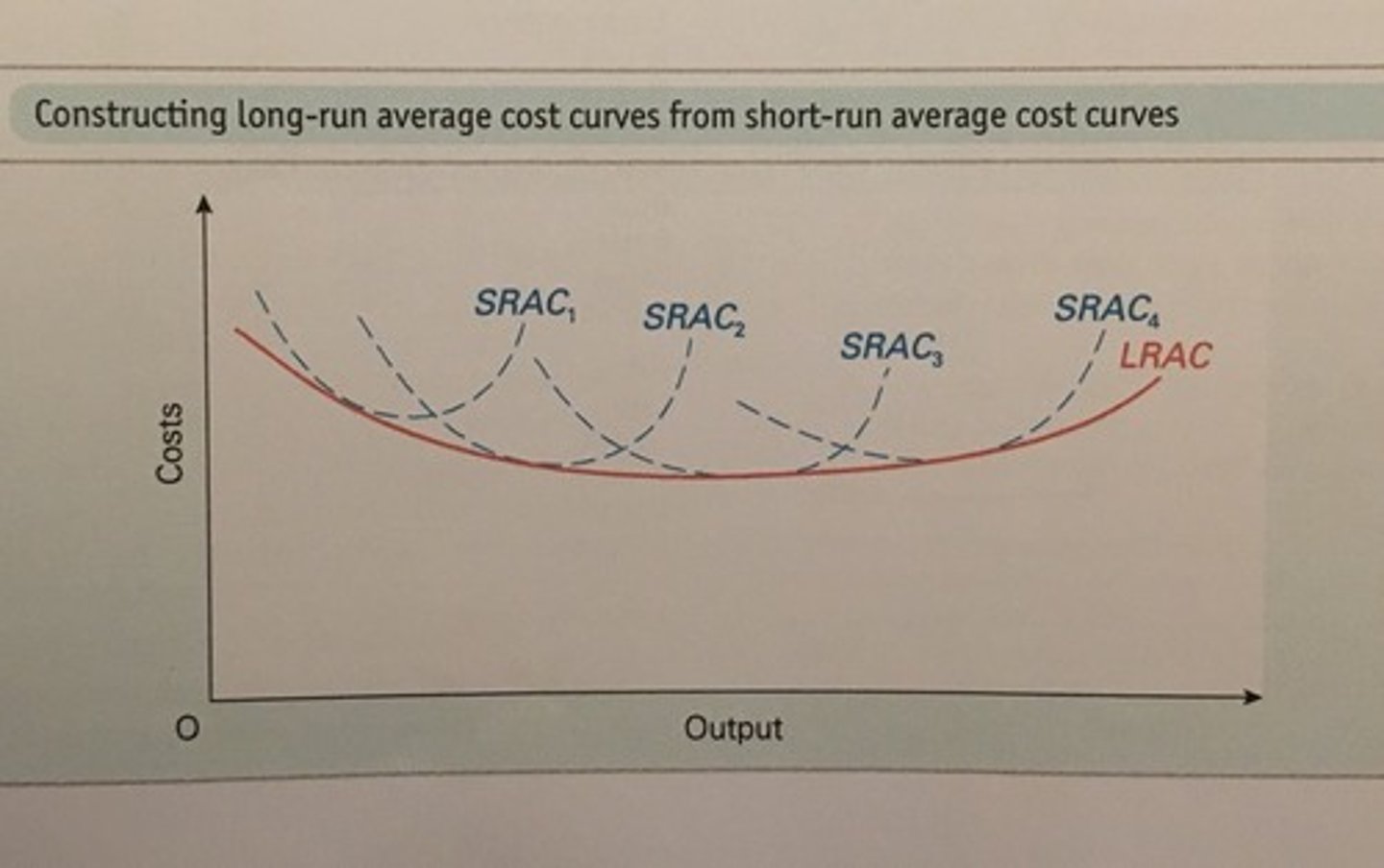
Long Run Average Cost (LAC)

a firm's long-run total cost divided by output

short run average cost (SAC) (SRAC)

a firm's total cost per unit of output when it has one or more fixed inputs

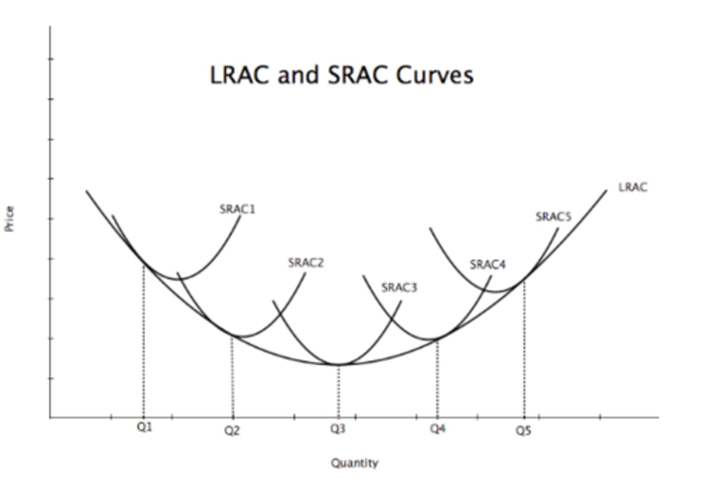
Short-run and long-run average costs

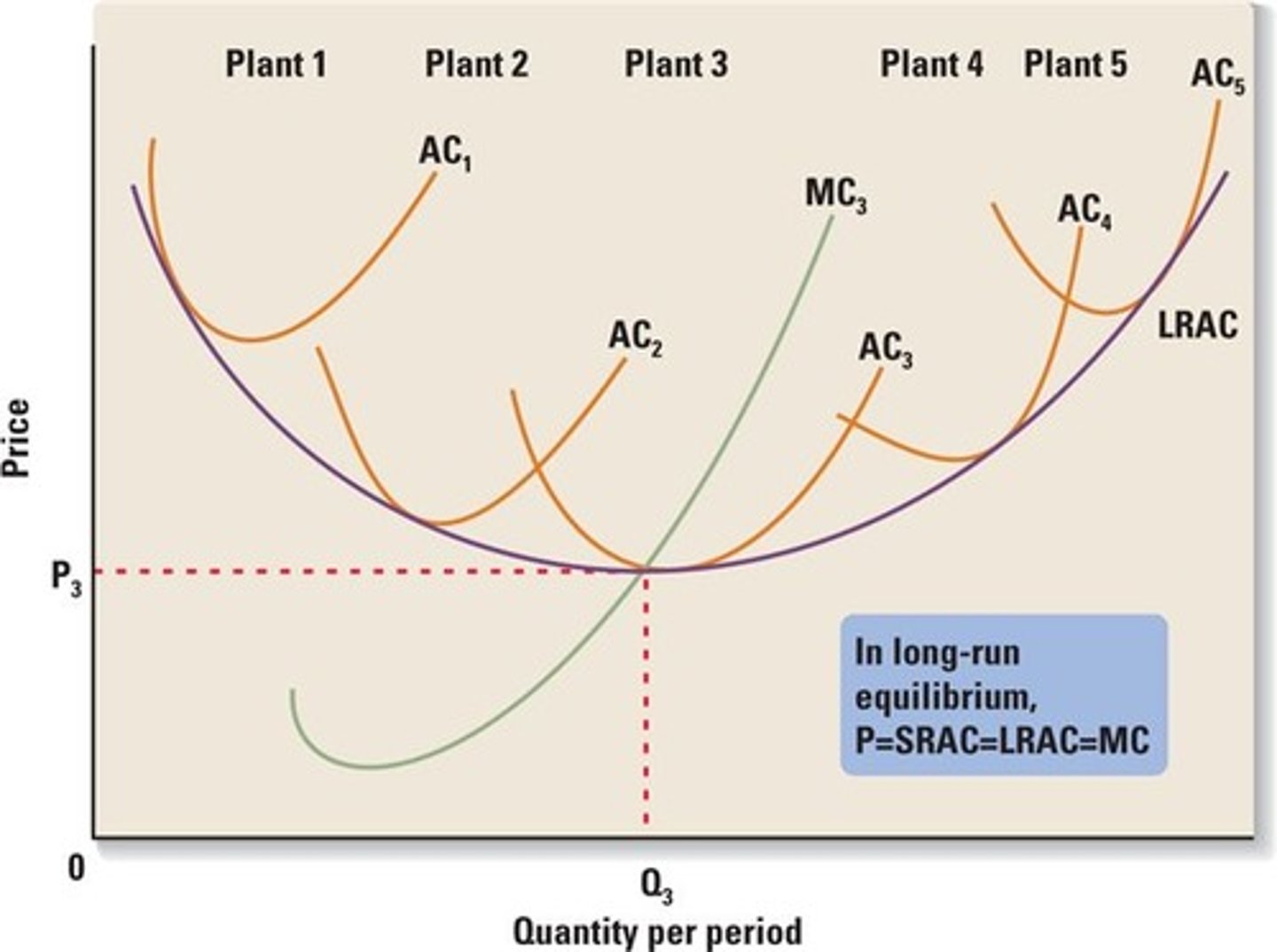
The short-run average cost (SRAC) curve(s) must be tangent to the long-run average cost (LRAC) curve.

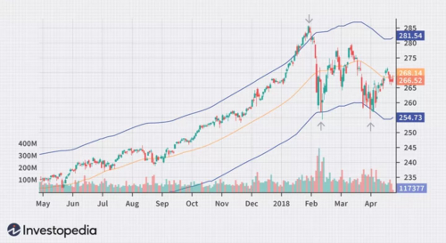
envelopes

technical indicators that are typically plotted over a price chart with upper and lower bounds

• The most common example of an envelope is a moving average envelope, which is created using two moving averages that define upper and lower price range levels

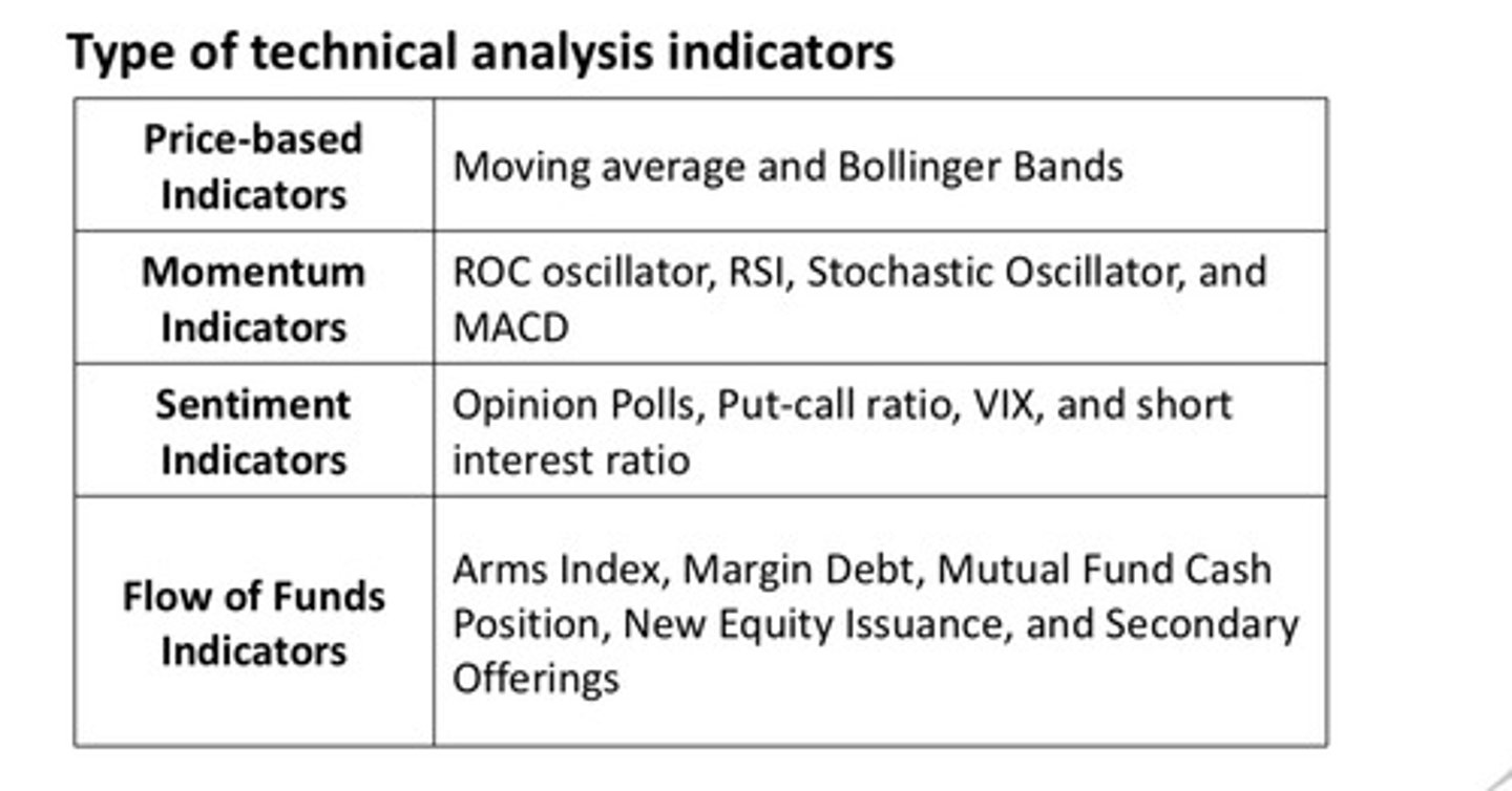
Technical Indicators

Mathematical formulas designed to be added to charts to assist with technical analysis of trends, momentum and volatility.

• Relative Strength Index (RSI)

• Money Flow Index (MFI)

• stochastics

• moving average convergance divergence (MACD)

• Bollinger Bands

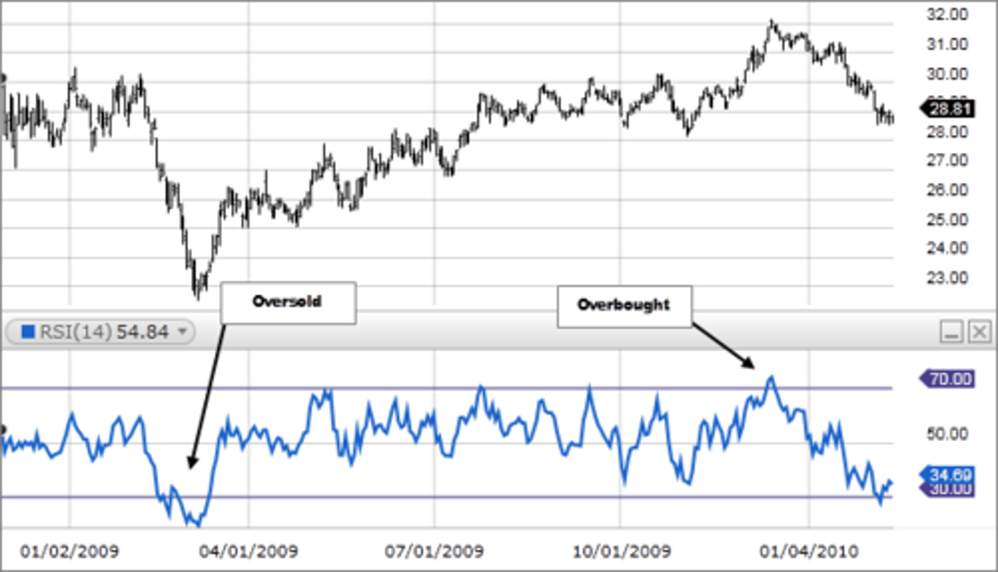
Relative Strength Index (RSI)

A momentum indicator that compares the magnitude of recent gains and losses over a specified time period to measure speed and change of price movements of a security

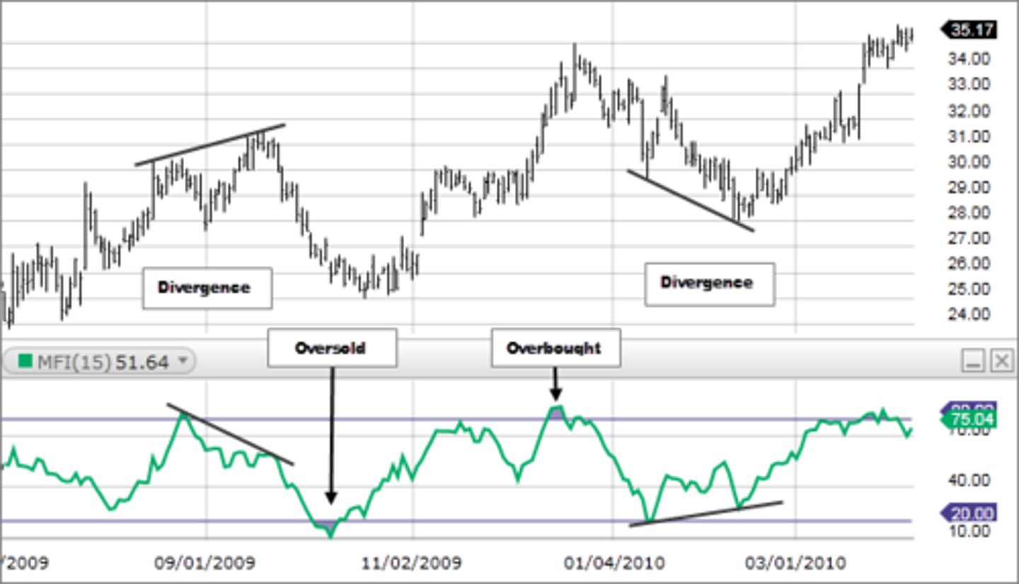
Money Flow Index (MFI)

a technical oscillator that uses price and volume data for identifying overbought or oversold signals in an asset. It can also be used to spot divergences which warn of a trend change in price.

• oscillator moves between 0 and 100

• think of it as volume-weighted version of RSI that shows shifts in buying and selling pressure

Stochastics

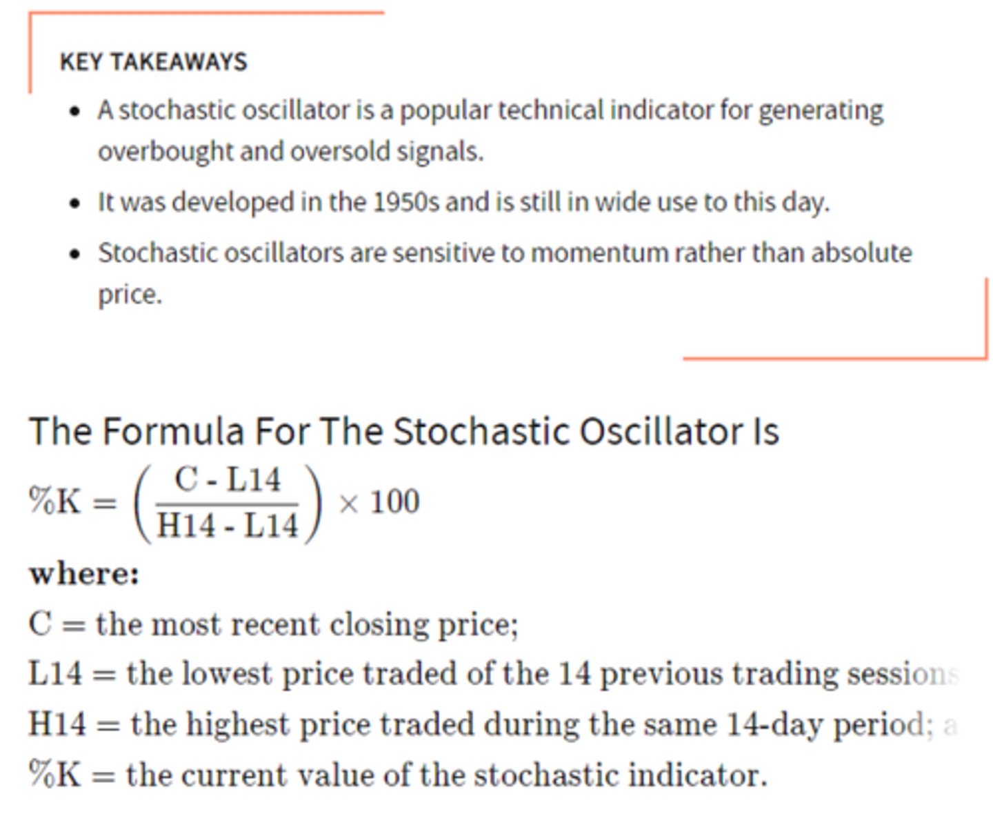
the tools and formulas of technical analysts measuring the momentum of stocks and stock indexes

Moving Average Convergence Divergence (MACD)

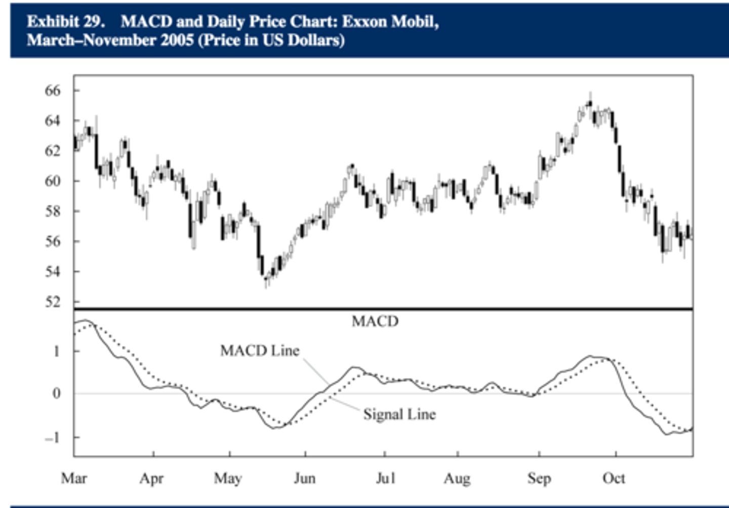
A technical analysis tool that takes the difference between two moving averages and then generates a smoothed moving average on the difference (the divergence) between the two moving averages; a trend-following momentum indicator that shows the relationship between two moving averages of a security's price

Bollinger Bands

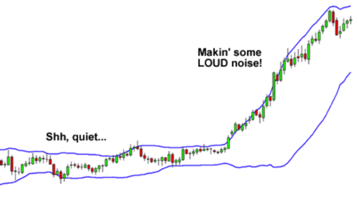
a technical analysis tool defined by a set of trendlines plotted two standard deviations (positively and negatively) away from a simple moving average (SMA) of a security's price, but which can be adjusted to user preferences

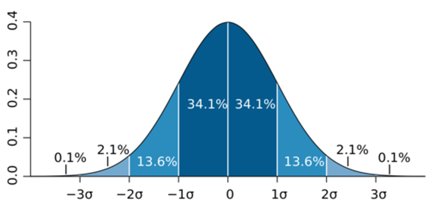
Standard Deviation (SD)

A measure of variability that indicates the average difference between the scores and their mean

The long-run average cost curve is the _____ envelope of the short-run average cost curves.

lower

• The short-run average cost curve must be tangent to the long-run average cost curve

• Say there were four plants working under a single entity and were producing the same kind of output, but at different rates. Each short-run cost curve associated with that plant would be tangent to the long-run average cost curve.

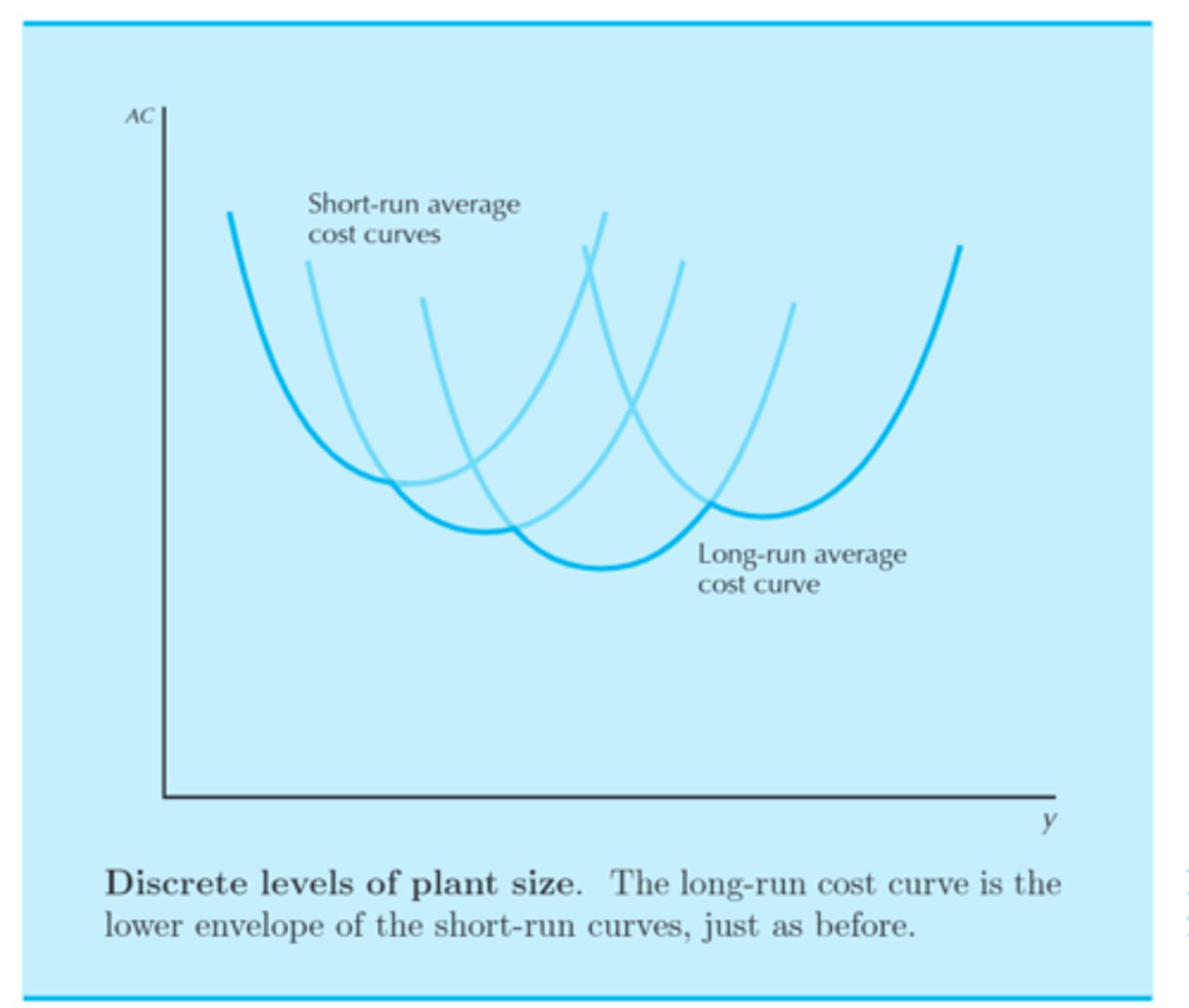
Discrete levels of plant size

Say there are multiple plants working under a single entity and are producing the same kind of output, but at different rates. Now consider that these plants have discrete levels of sizes, rather than continuous.

The long-run cost curve is the lower envelope of the short-run curves, much like with factories that have continous levels of plant sizes.

• see diagram

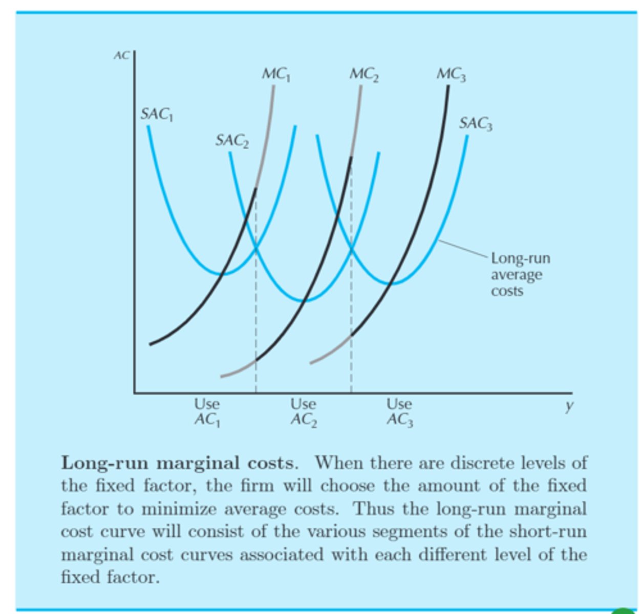
The long-run _______ ____ at any output level, y, has to equal the short-run marginal cost associated with the optimal level of plant size to produce y level of output.

marginal cost

long-run marginal cost (LMC)

The change in long-run cost resulting from a one-unit increase in output

• When there are discrete levels of the fixed factor, the firm will choose the amount of the fixed factor to minimize average costs. Thus the long-run marginal cost curve will consist of the various segments of the short-run marginal cost curves associated with each different level of the fixed factor.

Which of the following statements are true?

(1) Average fixed costs never increase with output.
(2) Average total costs are always greater than or equal to average variable costs.
(3) Average cost can never rise while marginal costs are declining.

1) true
2) true
3) false

A firm produces identical outputs at two different plants. If the marginal cost at the first plant exceeds the marginal cost at the second plant, how can the firm reduce costs and maintain the same level of output?

By simultaneously producing more output at the second plant and reducing production at the first plant, the firm can reduce costs.

Is the following statement true or false?

"In the long run a firm always operates at the minimum level of average costs for the optimally sized plant to produce a given amount of output."

FALSE