Sampling distributions and difference in means

Sampling distributions and difference in means

Sampling Distributions

• is the probability distribution of a statistic (e.g., mean, proportion) from multiple samples.

Probability

• is a measure of the certainty associated with a future event or occurrence and is usually expressed as a number between 0 and 1 (or between 0 % and 100 %).

How to measure probability?

P (A) = Number of favourable cases/ Number of possible cases

P (A) = Number of times A occur/ Number of times A can occur

Example of probability measurement

Coin toss (A).

P (A) = 1/2 = 0,5

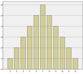
Characteristics of normal distribution of mean and variance

1. Being bell-shaped, mesocturtic.

2. Being symmetric

3. Coincide mean, median and mode = central tendencies

4. Having 95% of the indicators within the interval mean +- 2 standard deviations.

Central Limit Theorem (CLT)

• The distribution of the sample mean approaches a normal distribution as sample size increases (n ≥ 30).

• Mean of sampling distribution = population mean (µ).

• Standard deviation of sampling distribution = standard error (SE).

Estimator

• Is a function of the values in the sample.

• Estimators can be calculated with the sample

Parameter

• population

Normal distribution is indicated for data

• follow a continuous scale: weight, height, age, cholesterol, blood pressure, uric acid

• It has the advantage that under certain conditions

Law of large numbers

states that as a sample size increases, the sample mean (x-bar) gets closer to the population mean (µ)

There are two types of Law of Large Numbers

• Weak Law

• Strong law

Weak law

Sample mean converges in probability to the population mean.

Strong law

Sample mean converges almost surely to the population mean.

Implications of Law of Large Numbers

• Larger samples provide more accurate estimates of population parameters.

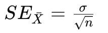
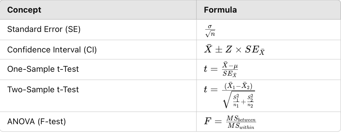
Standard Error (SE) formula for mean

• = Population standard deviation

• = Sample size

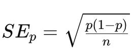
Standard Error (SE) Formula for proportion

p = Population proportion

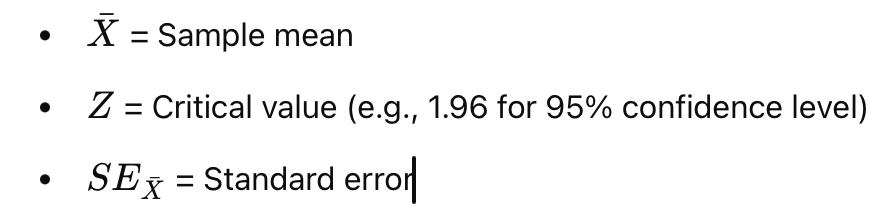
Confidence Intervals (CI)

• gives a range of values where a population parameter likely falls.

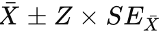
Formula for CI of the Mean

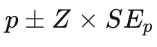
Formula for CI of Proportions

Hypothesis Testing for Means

1. State null (H₀) and alternative (H₁) hypotheses.

2. Select significance level (∂., usually 0.05).

3. Calculate test statistic (z or t-score).

4. Compare with critical value OR find p-value.

5. Decide: Reject H₀ if test statistic > critical value OR p-value <∂. (alfa)

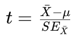
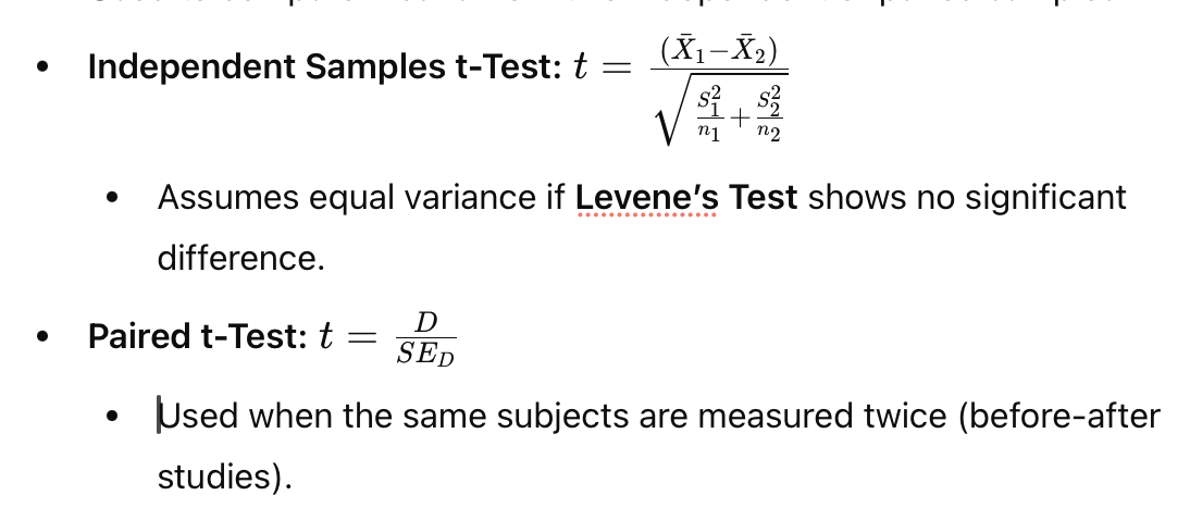
• t-Test Formula for Mean Comparison

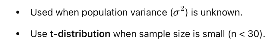
Comparing Two Means

Used to compare means from two independent or paired samples.

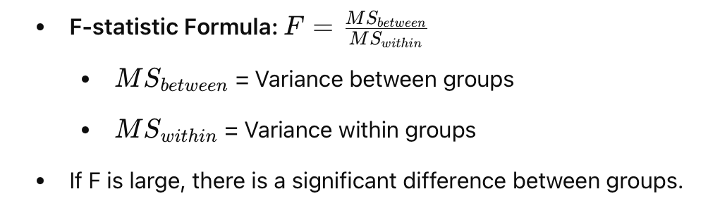
ANOVA (Analysis of Variance)

• Used to compare more than two means

Assumptions for t-Tests & ANOVA

1. Normality – Data should be normally distributed.

2. Independence – Samples should be independent.

3. Homogeneity of Variance – Variances should be equal across groups (check with Levene’s test).

Concepts & formulas

PROBABILITY  - normal distribution

DESCRIPTIVE STATISTICS

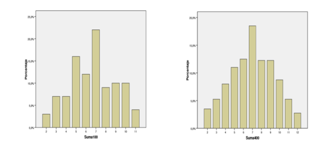
Central Limit Theorem

• states that sample distributions approach the normal distribution as the sample size increases.

• This means that very small sample sizes can cause problems in approximating a normal distribution.

• If X is a random variable of any distribution, with a large sample size (n > 30), it follows approximately a normal distribution.

• This property is valid whatever the random variable

Analysis of normality

Parametric

Non-parametric

Parametric

A variable is considered parametric if it follows a normal distribution

Non-parametric

• a variable which does not follow a normal distribution

• This is especially important when defining the statistics in statistics.

• Inferential

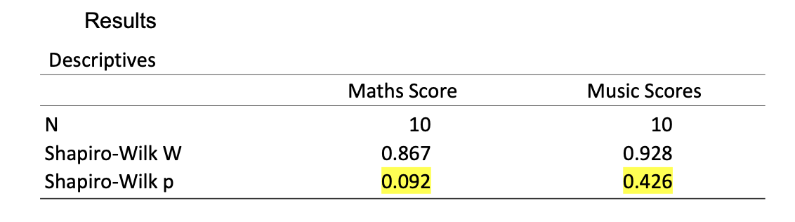
Shapiro-Wilk

• If p > 0.05 it means that the distribution is normal, which means that it is considers a parametric variable

Example of Shapiro-Wilk

Distribution of averages

• Set of "averages" of samples of a given size that have been drawn from a population.

• It is the distribution (data set) of reference when we do a hypothesis test on a sample or more than one person.

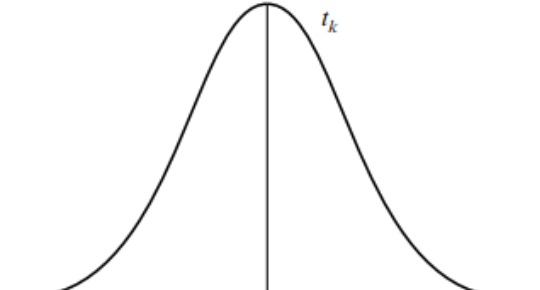
Distribution model (normal distribution) Student's t-distribution

• Symmetric with respect to the value 0, where the indices of central tendency coincide (unimodal).

• Can take positive and negative values

• Asymptotic about the abscissa axis

• There is a whole family of T-distributions depending on their degrees of freedom (l.g.).

• As the l.g. increases, the dis

• parametric test to analyse it

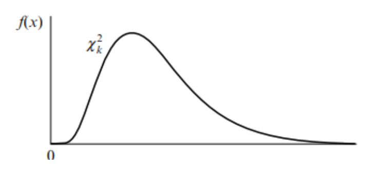
Pearson's x2 distribution

• Cannot take negative values

• Positive asymmetric

• There is a whole family of distributions depending on their degrees of freedom (l.g.).

• Right-hand asymptotic only

• As the l.g. increases, the distribution becomes closer to normal.

• Non-parametric distribution

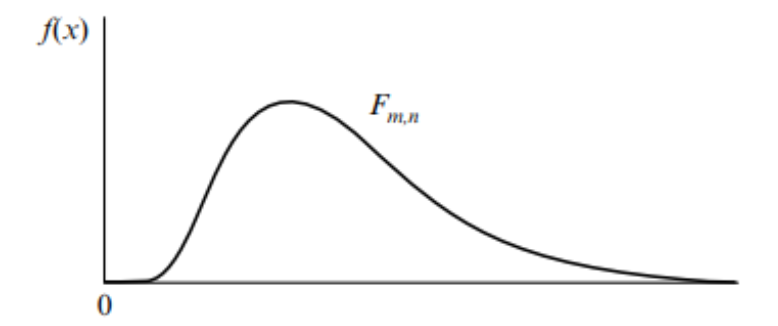
Snedecor F distribution

• Cannot take negative values

• Positive asymmetric

• There is a whole family of distributions depending on their degrees of freedom (l.g.) in numerator and denominator.

• Right-hand asymptotic only

• As the l.g. of numerator and denominator increase, the distribution becomes closer to normal.

• Non-parametric distribution