Review-Ch 5 Statistics

Probabilities

Probabilities

the long run frequency of an event

Probability Rules

1. ANY Probability is 0≤p(x)≤1

2. SUM of ALL probabilities is p(sum)=1

• complement event, event’=1-p(event)

  p(x^c)=1-p(x)

• the ‘ and power of c means the notation for the even not occurring

Law of Large numbers

• in the long run, a cumulative relative frequency is closer and closer to the true probability of an event

• random sampling, the larger the sample, the closer the proportion of success will be to the proportion of the population.

Simulation Process

1. Assumptions

   ______ selected independently of EACH other

   ____%

2. Assign digits & Model

• Number 01-99, ignore 00 and excess

• Numbers 00-99

• single run

• WHICH/HOW summary statistics will be recorded

3. Stimulate multiple/many repetitions

• Record results in a frequency distribution

4. conclusion

• Make sure it is in context

• estimated probability as a decimal

*Try to write EVERY possible outcome

*flip sign and +- SAME constant from mean→ SAME probability

Multiplication Principle

• The TOTAL possible outcome n_a wants x n_b way

• Sampling with/without replacement

Math

Independent: P(A) P(B)

Dependent: P(A) * P(B | A)

Conditional Probability

• May NEED to restrict in denominator values because of the “given that” → shrinks the population of interest

Math

P(__| __): given that

Mutually Exclusive

• Events that cannot occur simultaneously

• doesn’t imply independence

• can ADD Probabilities

Independant events

• Results don’t affect EACH other

• can multiply probabilities

• can be assumed for large populations

Dependent events

• EXPLICITLY write down EACH value/trial because results affect each other

Formula for mutually exclusive or not

Not mutually exclusive	Mutually exclusive
p(AUB)=p(A)+p(B)-p(A∩B)	p(AUB)=p(A)+p(B)

the mutually exclusive is because p(A∩B)=0 because events can’t happen at the SAME time

p(A∩B)

Probability of A and B

Independent:p(A∩B)=p(A)*p(B)

Dependent: (A∩B)=p(A)*p(A|B)

p(A U B)

Probability of A or B

Independent: p(A)+p(B)-p(A∩B)

Dependent: NONE

p(A|B)

Probability of A given that B

Independent: p(A)

Dependent: p(A∩B)/p(B)

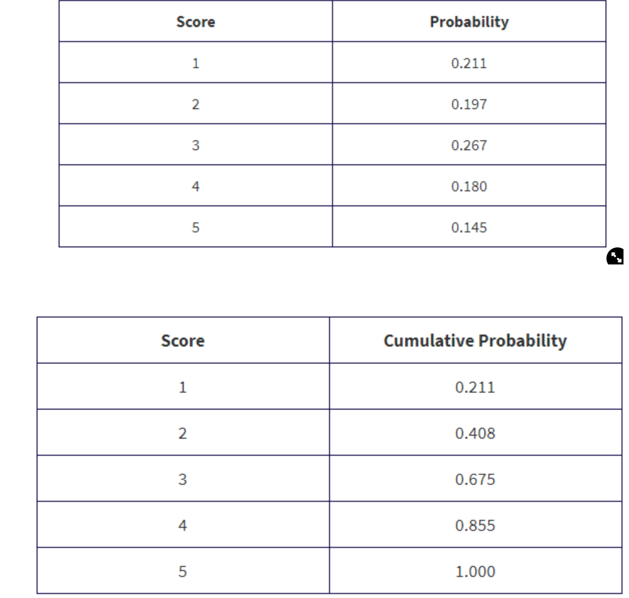
Probability distribution

• the number of practical outcomes of a CHANCE process

• follows probability rules

• set number of trials

• x variable =number of success

• Scenarios

  • if not ALL values are EXPLICITLY shown for probability → calculate what you can to solve

  • only several values, not all→ consider minimum, mean/median, maximum

Expected value

• the net value on average

Math

u_x=E(x)=np

u_x

• the mean of x variable

Math

u_x=Σxi *p(xi)

σ _x

• the stndard deviation of x variable

σ _x= √ (Σxi - u_x )²*p(xi)

sq root all

( σ _x)²

• variance

finiding z score through norrmal distribution

1. invnorm

• given the % of area

• using (o,1) as (u,σ ) for the default

2. Z formula

• z=(x-u)/σ

C (Linear transformation )

C=shift in +-

• only affects the mean

Math

u_c+dx=|d|u_x+c

σ _c+dx=|d|σ_x

D(Linear transformation )

• A transformation of *

• affects BOTH the mean and the standard deviation

Math

u_c+dx=|d|u_x+c

σ _c+dx=|d|σ_x

u mean (Combining sets)

• u can also mean E(x), the expected vlalue

Math

u_x+y=u_x+u_y

u_x-y=u_x-u_y

σ standard deviation (Combining sets)

• for the formulas, need to be √ and have ² inside because standard deviations are ALWAYS positive

Math

σ_x+y=√(σ²_x+σ²_y)

σ_x-y=√(σ²_x-σ²_y)

σ² varience (Combining sets)

• Usually, a NEW variable is created which represents a total

• remove the √ because variance is standard deviation ²

Math

σ²_x+y=(σ²_x+σ²_y)

σ²_x-y=(σ²_x-σ²_y)

Linear Combination

• when constants are multiplied in

• for mean, just multiply in

• for sd and variance, need to square values

Math

u= au_x+bu_x

σ=√a²σ_x²+ b²σ_y²

σ²=a²σ_x²+ b²σ_y²

Binomial Distribution (Definition)

BINS

B: Binary(2 outcomes ONLY)

I: Independent(outcomes don’t affect impact EACH other)

N: Number of trials is FIXED

S: Success probability (is constant)

• as n, the number of trials, increases→ shape of distribution becomes MORE normal

Binomial Distribution (steps)

STEPS

1. Name the distribution(ie. binomial…)

2. Set Parameters(ie. n=, p=)

3. Boundaries(eg. at least…)

4. Direction(inequalities signs)

5. Correct probability

Binomial Distribution (formula’s)

Math

u_x=np

σ_x√=np(1-p)

σ_x²=np(1-p)

• at p=0.5→ variance increases as n increases

• fixed n value, V is the maximum when p=0.5

Geometric Distribution (Definition)

BINS

B: Binary(2 outcomes ONLY)

I: Independent(outcomes don’t affect impact EACH other)

N: Number of trials is not FIXED

S: Success probability (is constant)

• random variable, x, COUNTS trial NO. until the first success

  *most likely value is 1

• expected trials till n^th success = np

• the probability of EACH success value decreases by a factor of q= 1-p

• Shape: ALWAYS unimodal and skewed right

Geometric Distribution (steps)

STEPS

1. Name the distribution(ie. geometric…)

2. Set Parameters(ie. p=)

3. The trial on which the first success occurs(x=)

4. Correct probability

Geometric Distribution (formula’s)

Math

• q=fail, p=success

q=1-p

u_x= 1/p

σ_x= (√ 1-p)/p

Probability that the 1st success occurs on the x^th outcome

p(x=_)=geompdf(p= ,x=)

• p=probability of a single trial, = first success occurrence

more than x tries till first success(calculator)

p(x>_)=1- geomcdf(p= ,x=)

• the 1- and the x=number means everything “ABOVE”

cumulative probability of x or BEFORE x^th trail

p(x=_)=1geomcdf(p= ,x=)

• p=probability of a single trial, = first success occurrence

• n is not given→leave empty

• “First success occurrence ON or BEFORE x^th trail”

Probability of exactly x success

binompdf(n,p,x)

• n=total no. of trial

• p=probability of success of a single trial

• x=number of wanted success’s

Cumulative probability of f or FEWER success in n ways

binomcdf(n,p,x)

• n=total no. of trial

• p=probability of success of a single trial

• x=c or fewer success

At least… binom

p=(x≥number)

1-binomcdf(n=,p=,x=number-1)

fewer than…

(x<number)

binomcdf(n=,p=,x=number-1)

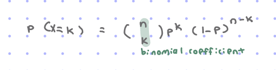
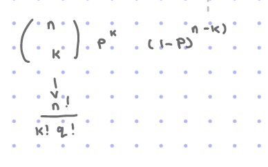
interpret the formula for binomial

(n on top of p) = n!/(k!q!)

• n=total trial no.

• k=wanted

• p=probability

• q=p-1

Sample space

• set of ALL possible outcomes

• ie {H, T}

Event

• Outcome OR set of outcomes of a random thing

Probability model

• Assign probabilities to EACH event inn sample space

• example

  • p(tails)=0.5

  • p(heads)=0.5

Random

• A regular pattern can be inferred if long repetitious trials are run, but for individual outcomes→this is uncertain

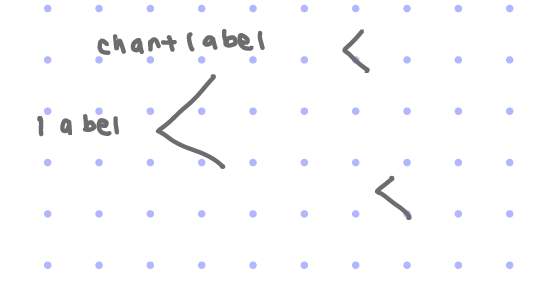
Tree diagram

• used for multi step problems

• Label the start and then < grow on

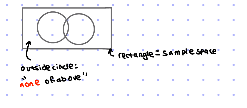
Venn diagrams

• intersections overlap→ don’t “repeat” them, so may need to use subtraction

• outside circle: “none of above”

• rectangle box=sample space

U

add, union

∩

• or

• 1 event or BOTH occurring

Relative frequency

• proportion of times the event happened

number of times event happened/total number of trials

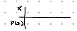
Cumulative probability distribution

• A function, table, or graph that links outcomes with the probability of less than or equal to that outcome occurring.