Module 10 Decision Analysis, Expected Value Approach, anf AHP

Regret is the difference between the payoff associated with a particular decision alternative and the payoff associated with the decision that would yield the most desirable payoff for a given state of nature. T or F?

True

The decision alternative with the best expected monetary value will always be the most desirable decision. T or F?

False

The expected value approach is more appropriate for a one-time decision than a repetitive decision. T or F?

False

The expected value of an alternative can never be negative. T or F?

False

The primary value of decision trees is that they provide a useful way to organize how operations managers think about complex multiphase decisions. T or F?

True

Lakewood Fashions must decide how many lots of assorted ski wear to order for its three stores. Information on pricing, sales, and inventory costs has led to the following payoff table, in thousands.

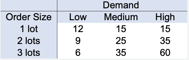
Part a) ​Which ​of the following decision trees correctly represent the problem described above?

Part b) What decision should be made by the optimist, i.e., someone using the Maximax Approach?​

Order 2 lots

Order 1 lot

Order 3 lots

Order 3 lots

Part c) What decision should be made by the conservative, i.e., someone using the Maximin Approach?​

Order 2 lots

Order 1 lot

Order 3 lots

Order 1 lots

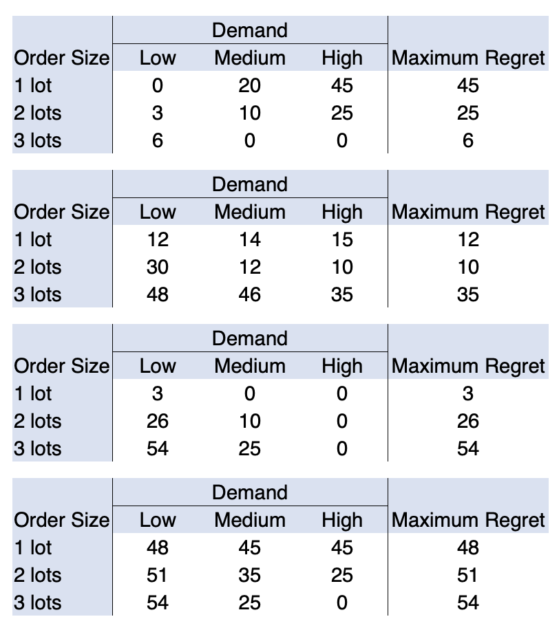
Part d) For each state of nature, calculate the regret of each choice. Which one of the following is the correct regret-table?

first table

Part e) What decision should be made using minimax regret?

order 3 lot

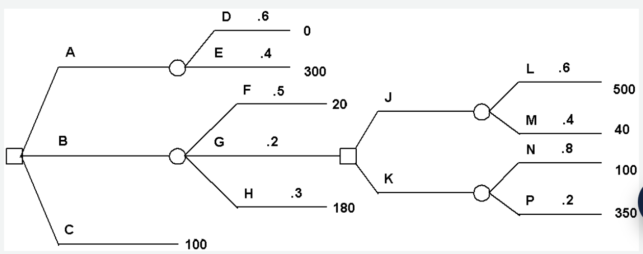
Determine decision strategies based on expected value for this decision tree.

Part a) What is the expected value after branch A, i.e., EV(A) =?

Branch A leads to a chance node with two outcomes:

• D with probability 0.6 → payoff 0

• E with probability 0.4 → payoff 300

So:

EV(A)=(0.6)(0)+(0.4)(300)EV(A)=(0.6)(0)+(0.4)(300)EV(A)=0+120=120EV(A)=0+120=120​

Part b) What is the expected value after branch J, i.e., EV( J ) =?

Branch J leads to a chance node with two outcomes:

• L with probability 0.6 → payoff 500

• M with probability 0.4 → payoff 40

• EV(J)=(0.6)(500)+(0.4)(40)

• Compute each part:

  • 0.6×500=3000.6×500=300

  • 0.4×40=160.4×40=16

  • EV(J)=300+16=

• 316

Part c) What is the expected value after branch K, i.e., EV( K ) =?

150

Part d) What is the expected value after branch B, i.e., EV( B ) =?

Hint: Use the information you calculated before, i.e. EV( J) and EV( K). Use the most favorable outcome.

• EV(J) = 316

• EV(K) = 150

• EV(B)=max(316,150)=316​

Part e) What is the expected value after branch C, i.e., EV( C ) =?

100 there are no outcomes associated with branch C, meaning it has no expected value.

Part f) Based on the maximum expected value approach, what should be the initial decision strategy?

Select decision alternative C

Select decision alternative B

Select decision alternative A

Select decision alternative B

 max(120, 316, 100)=316

Part g) Suppose that initially decision alternative B is selected and then G happened. Based on the maximum expected value approach, what should be the next decision strategy?

Select decision alternative J

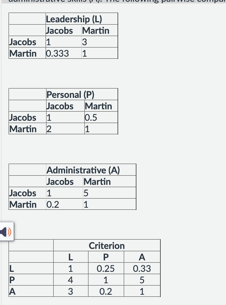
he vice president of Harling Equipment needs to select a new director of marketing. The two possible candidates are Bill Jacobs and Sue Martin, and the criteria thought to be most relevant in the selection are leadership ability (L), personal skills (P), and administrative skills (A). The following pairwise comparison matrices were obtained:

Part a) The column totals of the criteria comparison matrix are:

Leadership column total = 8

Personal column total = 1.45

Administrative column total = 6.33

Leadership column values:

• From L row → 1

• From P row → 4

• From A row → 3

1+4+3=81+4+3=8

Personal column values:

• From L row → 0.25

• From P row → 1

• From A row → 0.2

0.25+1+0.2=1.450.25+1+0.2=1.45

Administrative column values:

• From L row → 0.33

• From P row → 5

• From A row → 1

0.33+5+1=6.330.33+5+1=6.33

Leadership column total = 8
Personal column total = 1.45
Administrative column total = 6.33

Part b) If you divide each cell in each column by the column total you get the Normalized Pairwise Comparison Matrix for the Criteria:

the 4th option 

Divide each value by 8:

• L row: 1/8=0.1251/8=0.125

• P row: 4/8=0.5004/8=0.500

• A row: 3/8=0.3753/8=0.375

Divide each value by 1.45:

• L row: 0.25/1.45≈0.1720.25/1.45≈0.172

• P row: 1/1.45≈0.6901/1.45≈0.690

• A row: 0.2/1.45≈0.1380.2/1.45≈0.138

• Divide each value by 6.33:

  • L row: 0.33/6.33≈0.0520.33/6.33≈0.052

  • P row: 5/6.33≈0.7905/6.33≈0.790

  • A row: 1/6.33≈0.1581/6.33≈0.158

  • Criteria	Leadership	Personal	Administrative
    Leadership	0.125	0.172	0.052
    Personal	0.500	0.690	0.790
    Administrative	0.375	0.138	0.158

Part c) What are the criteria priorities (row averages on normalized comparison matrix)?

Criteria Priorities 

	Row Average
Leadership	0.117
Personal	0.660
Administrative	0.224

Part d) Compute the priorities for the Leadership pairwise comparison matrix. We will go step by step.

	Leadership
	Jacobs	Martin
Jacobs	1	3
Martin	0.333	1

Step 1: Column totals

Step 2: Normalized Pairwise Comparison Matrix (see slides and Excel for an example)

Step 3: Calculate row average

Jacobs column total1+0.333=1.333

1+0.333=1.333

Martin column total

3+1=4

3+1=4

Part e) Compute the priorities for the Leadership pairwise comparison matrix. We will go step by step.

	Leadership
	Jacobs	Martin
Jacobs	1	3
Martin	0.333	1

Step 1: Column totals

Step 2: Normalized Pairwise Comparison Matrix (see slides and Excel for an example)

Step 3: Calculate row average

Normalized Pairwise Comparison Matrix

	Leadership
	Jacobs	Martin
Jacobs	0.750	0.750
Martin	0.250	0.250

Part f) Compute the priorities for the Leadership pairwise comparison matrix. We will go step by step.

	Leadership
	Jacobs	Martin
Jacobs	1	3
Martin	0.333	1

Step 1: Column totals

Step 2: Normalized Pairwise Comparison Matrix (see slides and Excel for an example)

Step 3: Calculate row average

Row Averages

	Leadership
	Jacobs	Martin	Row Average
Jacobs	0.750	0.750	0.750
Martin	0.250	0.250	0.250

Part g) Now, this time compute the priorities for the Personal pairwise comparison matrix. We will again go step by step.

	Personal
	Jacobs	Martin
Jacobs	1	0.5
Martin	2	1

Step 1: Column totals

Step 2: Normalized Pairwise Comparison Matrix (see slides and Excel for an example)

Step 3: Calculate row average

Part l) Based on the overall priority calculations you do in Part k), what is Jacobs' score =

0.494

Part m) Based on the overall priority calculations you do in Part k), what is Martin's score =

0.506

In the Analytic Hierarchy Process (AHP), why is the Consistency Ratio (CR) important when evaluating pairwise comparisons?

It measures how much the final priorities depend on the number of alternatives.

It ensures that all criteria are equally weighted.

It checks whether the decision maker’s judgments are logically consistent with each other.

It increases the accuracy of the eigenvalue calculation.

It checks whether the decision maker’s judgments are logically consistent with each other, helping to validate the reliability of the priority outcomes.

A decision maker prefers A > B, B > C, and C > A in their pairwise comparisons. How could this inconsistency affect AHP?

It could increase the Consistency Ratio (CR) above the acceptable level.