Linear Regression

predicted value (y hat)

The estimate made from the model

Residual

The difference between the observed value (the one that’s given) and the predicted value (using model) and it tells us how far off the model’s prediction is at that point

To find residuals

residual = observed - predicted (y- y hat)

If there’s a patter in the residual plot..

then the model is not appropriate

a line that fits well has..

very small residuals

How to asses how well the line fits with residuals?

squaring the residuals (makes them all positive and emphasizes large residuals)) and then adding them all up (the smaller the sum the better)

Least Squares Line or the Least squares regression line (LSRL)

the unique line of a data set that makes the sum of the squared residuals as small as it can be

Correlation and Line

Correlation and the line are related. The correlation leads us to the equation we need to model the data

What r tells us about the regression

• For each SD of x that we are away from the x mean, we expect to be r SDs of y away from the mean

• Because r is always between -1 and +1, each predicted y is fewer SDs away from its mean than the corresponding x was (regression to the mean)

• The slope of the line is based on the correlation (slope = r times the quotient of SD of y divided by SD of x)

Regression to the mean

each predicted y tends to be closer to its mean (in SDs) than its corresponding x was.

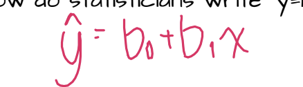
Line of best fit/ LSRL formula

y hat= bo +b1x

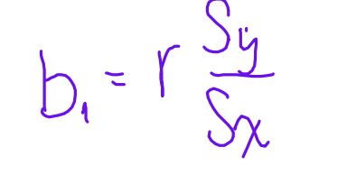
slope formula

b1 = r times sy divided by sx

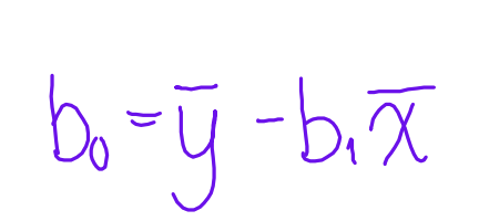
y-intercept formula

b0 = average y - b1 times average x

slope

as your explanatory variable increases by ___ the response variable has been associated by an increase of b1 (NOT CAUSE AND EFFECT)

y-intercept

when explanatory variable is 0, the response variable is b0

Typical Residual Size/ Standard Error

one way to evaluate how good a model is, a rough estimate of how much our model is typically off by when we use it to predict the y-values from the x-values

Standard Error formula

Standard error= standard error of residuals= difference between y and y hat, squared and summed up, then divide by n-2, then square root it

Coefficent of Determination (r²)

in general, when the LSRL is used to fit bivariate data, it represents the fraction of the variation between 0-1 (always positive because it’s squared); this tells you the % of the variation in the responses (= to how the % that the model explains the data), so the closer it is to 1 the better/more robust the model is.

A tale of 2 regressions

you CANNOT PREDICT X FROM Y IN A MODEL because they have different equations (but same correlation, but need to switch variables to get new regression)

Before starting a regression, check the following things:

• Quantitative Variable Condition (are both variables quantitative?)

• Straight Enough Condition (is r and r² close to 1/ is the data straight and linear enough to run a regression)

• Outlier Condition

• Does the plot thicken? (make sure there’s a relatively consistent spread (also for residuals)

• Check the residuals with residual plot (if there’s a pattern = linear model is NOT APPROPRIATE even with high r/r²)

What can go wrong?

• Don’t force a linear relationship

• Don’t say x causes y

• Don’t invert regression

• Don’t choose based off r²/scatterplot alone (check EVERYTHING to make sure that the model is appropriate)