Analogue to Digital Filtering, The sampling process, Aliasing, Reconstruction, Principles of Digital Filtering (2 - 2.2)
1/14
There's no tags or description
Looks like no tags are added yet.
Name | Mastery | Learn | Test | Matching | Spaced |
|---|
No study sessions yet.
15 Terms
What is the difference between analogue and digital filters?
Analogue filters are built using components like resistors, inductors, and capacitors. Digital filters, on the other hand, are implemented in hardware or software using numerical processors such as CPUs or GPUs. Digital filters offer several advantages:
- Reprogrammability for different filters.
- Accuracy is dependent only on predictable round-off errors.
- Immune to power supply or temperature variations.
- Higher noise immunity compared to analogue filters.
How does digital filtering work in the time and frequency domains?
- In the time domain, digital filtering is performed by convolving the input signal with a digital impulse response.
- In the frequency domain, filtering involves multiplying the signal spectrum by the desired filter response, typically using the z-transform.
What is the sampling process?
Sampling converts a continuous-time signal f(t) into a discrete-time signal f[k] , where samples are taken at intervals t = kT .
- The sampling rate is f_s = \frac{1}{T} .
- A continuous-time sinusoidal signal with frequency f_a and angular frequency \omega_a becomes:
x_a(t) = A \cos(2\pi f_a t + \phi) \ \text{and} \ x_d[n] = A \cos(2\pi f_d n + \phi),
where f_d = \frac{f_a}{f_s} and \omega_d = \omega_a T .
What are digital and unique frequencies?
In discrete-time systems, two sinusoidal signals with angular frequencies differing by multiples of 2\pi are identical. Therefore, the digital angular frequency \omega_d lies in the range:
-\pi \leq \omega_d \leq \pi.
Similarly, the digital frequency f_d is unique within the range:
-\frac{1}{2} \leq f_d \leq \frac{1}{2}.
If you sample above this frequency, the resulting sampled waves will be copies of waves sampled at lower frequencies.
What is the Nyquist frequency?
The Nyquist frequency (or folding frequency) is the highest frequency in a continuous-time signal that can be uniquely represented after sampling. It is given by:
f_{\text{Nyquist}} = \frac{f_s}{2},
where f_s is the sampling rate. Any frequency higher than f_{\text{Nyquist}} will cause ambiguity due to aliasing.
By manipulating the inequality in the previous flashcard, we get,
-\frac{1}{2}f_s \leq f_a \leq \frac{1}{2}f_s.
This means sampling frequency is f_s, then the analogue signal must be less than half. It also shows the above statement about the highest frequency that can be represented from a sampling frequency.
What is aliasing in digital signal processing?
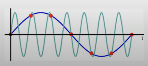
Aliasing occurs when different continuous-time signals produce identical sampled sequences. This happens because sampling introduces an ambiguity where frequencies outside the range [-f_s/2, f_s/2] appear as aliases within this range.
For example:
- A signal with f_a = 0.3f_s can be confused with f_a = 1.3f_s during sampling.
- This is because the sampled sequence is identical for these frequencies.
How can aliasing be understood from the frequency domain?
In the frequency domain, sampling a continuous-time signal causes its spectrum to repeat at intervals of the sampling frequency f_s.
- Frequencies beyond the Nyquist frequency f_s/2 overlap with those within [-f_s/2, f_s/2], causing aliasing.
![<p>In the frequency domain, sampling a continuous-time signal causes its spectrum to repeat at intervals of the sampling frequency $$f_s$$. </p><p>- Frequencies beyond the Nyquist frequency $$f_s/2$$ overlap with those within $$[-f_s/2, f_s/2]$$, causing aliasing.</p>](https://knowt-user-attachments.s3.amazonaws.com/7973fbae-d908-4f58-848c-fb20c0739a7d.png)
What is the solution to aliasing?
To avoid aliasing, the sampling frequency must be at least twice the maximum frequency present in the signal. This is called the Nyquist criterion.
Additionally, an anti-aliasing filter (e.g., a Butterworth low-pass filter) is applied before sampling to remove frequencies above f_s/2. This ensures that:
- Frequencies higher than f_s/2 are suppressed.
- The sampled sequence uniquely represents the original signal.
What is the reconstruction process in digital signal processing?
Reconstruction involves converting the processed digital signal back to a continuous-time signal. The process includes:
1. Digital-to-Analogue Conversion (DAC): Outputs discrete voltage levels corresponding to digital samples.
2. Interpolation: Fills the gaps between discrete samples. Common methods:
- Zeroth-order hold: Assumes the value of the sample remains constant until the next sample.
a. High-Frequency Artifacts: The signal created by the zero-order hold looks like a series of "steps" or "boxcars." These sharp transitions between steps create high-frequency noise or "artifacts." This happens because the sudden jumps in the signal introduce unwanted higher frequencies.
b. Attenuation of Low Frequencies: The signal produced by the zero-order hold also "flattens out" lower frequencies, meaning it weakens the smooth, slow variations in the signal. This is because of the shape of the signal's transition, which doesn't represent the smooth continuous signal well.
3. Output Low-Pass Filter (Recovery Filter): Smoothens the output and corrects distortions introduced by interpolation, such as:
- Smoothing spurious high-frequency components.
- Correcting low-frequency attenuation caused by the zeroth-order hold.
What is the role of the recovery filter in reconstruction?
The recovery filter achieves two objectives:
1. Smooths high-frequency replicas: Removes spurious components introduced during the reconstruction process.
2. Corrects low-frequency attenuation: Compensates for signal distortion caused by zeroth-order hold interpolation, which acts like a box function in the time domain and a sinc function in the frequency domain.
What is digital filtering?
Digital filtering involves the numerical processing of sampled signals to produce a "filtered" version. It can be thought of as a regression process, where noise reduction or smoothing is achieved by fitting mathematical models, like polynomials, to segments of the data.
What is parabolic filtering?
Parabolic filtering smooths data by fitting a parabola to every group of 5 data points in a sequence, and then selecting the central value of the fitted parabola. The parabolic approximation is computed using the current point and its 4 nearest neighbors. This forms a regression model that reduces noise.
How is the parabolic filter mathematically formulated?
The parabola for a group of 5 points is written as:
p[k] = s_0 + k s_1 + k^2 s_2,
where:
- p[k] is the value of the parabola at sample k ,
- s_0, s_1, s_2 are coefficients that fit the parabola to the data.
The coefficients are determined by minimizing the least-squares error:
E(s_0, s_1, s_2) = \sum_{k=-2}^2 (x[k] - (s_0 + k s_1 + k^2 s_2))^2.
What are the parabolic filter coefficients?
The coefficients s_0, s_1, s_2 are calculated by solving:
\frac{\partial E}{\partial s_0} = 0, \quad \frac{\partial E}{\partial s_1} = 0, \quad \frac{\partial E}{\partial s_2} = 0.
This yields the coefficients (we only need s_0 for the central value):
s_0 = \frac{1}{35}(-3x[-2] + 12x[-1] + 17x[0] + 12x[1] - 3x[2]),
s_1 = \frac{1}{10}(-2x[-2] - x[-1] + x[1] + 2x[2]),
s_2 = \frac{1}{14}(2x[-2] - x[-1] - 2x[0] - x[1] + 2x[2]).
What is the output of the parabolic filter?
The output sequence is given by the center point of the parabola, which is:
p[k] \big|_{k=0} = s_0.
This output is a smoothed approximation of the input data, with noise reduced due to the regression process. Each output value is based on 5 input points.