Unit 8 (STATS - 1000)

Summary of Learning Outcomes

• Confidence intervals and hypothesis tests for a population mean µ when ω is unknown

• Matched pairs t procedures

what did we assume in unit 6, and 7

we always assumed that we knew the population standard deviation, σ, of our variable of interest

Why is assuming we knew the population standard deviation unrealistic?

• This is an unrealistic assumption! In the real world, it’s unlikely we’d know the value of σ

• We’ve used this assumption so far only so that we can more easily explain the reasoning behind our methods

  • We are now ready to make the transition to the more realistic situation of unknown population standard deviation

How do we construct condfidence intervals

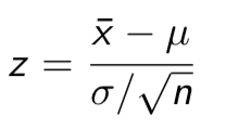
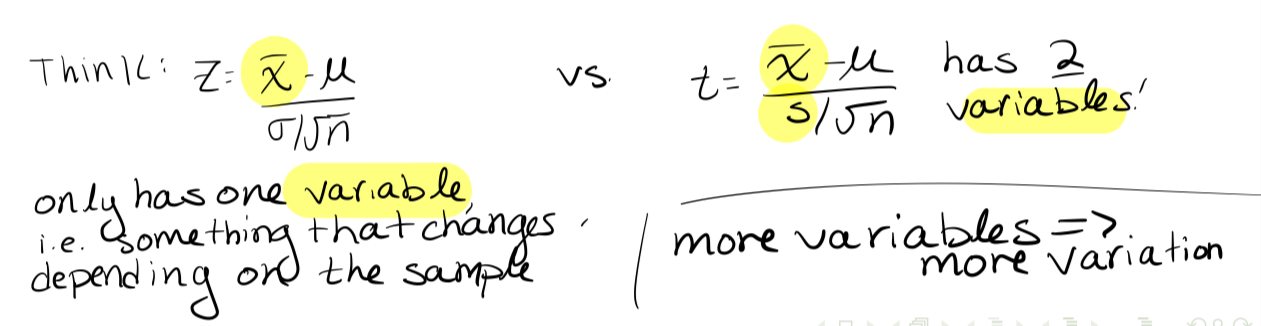
• In order to construct confidence intervals/perform hypothesis tests, we’ve needed to perform probability calculations with ¯X . To do this, we:

• transformed ¯X into Z , using the z-score formula, then

• used the Z table to find probabilities

  • If we don’t know the value of σ, then we can’t transform ¯X into Z. What should we do instead???

If we don’t know the value of σ, then we can’t transform ¯X into Z. What should we do instead???

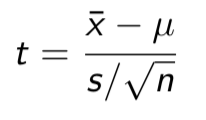
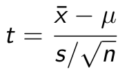
If σ is unknown, then we estimate it by the sample standard deviation s:

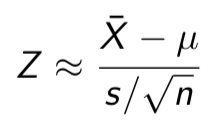
This standardized variable is very important, and so we give it its own name. If photo, then the variable

follows a t distribution

What is the quantity in the denominator of t called?

Standard error of the sample mean

What is the standard error of a random variable

Its estimated standard deviation

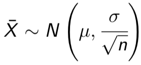
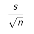
The true std.dev of ¯X Is σ/√n

If we don’t know σ, then our best estimate of the std.dev of ¯X Is s/√n

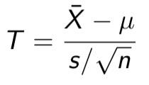
t - statistic

has a t distribution with n — 1 degrees of freedom.

What degree of freedom does the t - statistic have

It has n — 1 degrees of freedom.

What is degrees of freedom denoted as?

df

What does the shape of the t - distribution depend on

the sample size n:

• there is a di!erent t distribution for each possible value of n

How do we write the t - distribution with n - 1 degrees of freedom?

T(n - 1)

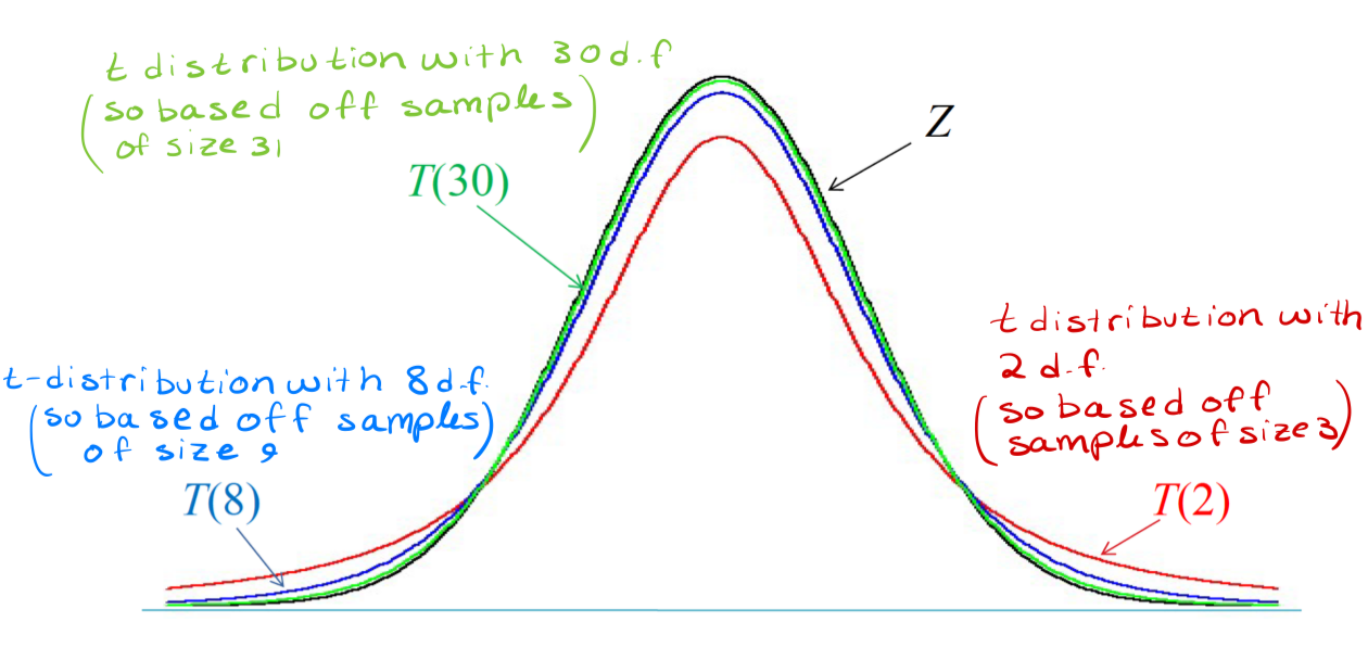
Since the form of T and Z are quite similar, we expect the shape of the t distributions to be similar to that of the standard normal curve

Symmetric about (T vs Z)

both symmetric about zero

Spread of the distribution (T vs Z)

The spread for t distribution is slightly greater than for the standard normal curve

• The t distributions have less area near the center and more in the tails than the standard normal distribution

• This is because estimating σ by s introduces more variation

Area location (T vs Z)

t distributions have less area near the center and more in the tails than the standard normal distribution

• This is because estimating σ by s introduces more variation

Formulas (T vs Z)

What happens as the degrees of freedom increases?

the t distribution approaches the standard normal distribution, Z

Why does the t - distribution approach the standard normal distribution z when df increases?

Because when n increases (and thus the degrees of freedom, n — 1 increases), s becomes a better estimate for σ! Thus T becomes closer to Z

When will we use t - distribution

t distribution (instead of Z ) to carry out methods of statistical inference (i.e. confidence intervals and hypothesis testing) when we don’t know the value of ω

t - distribution critical values

The critical values for selected t distributions are given in Table 2, for various confidence levels C (bottom row)/upper tail probabilities p (top row)

• The first column of Table 2 gives the degrees of freedom (df)

• The first row of Table 2 gives upper tail probabilities (i.e. areas to the right) different from Table 1 !!!

• The last row of Table 2 gives confidence levels C

• The entries in the body of the table give values of t* corresponding to a particular combination of degrees of freedom, and a particular confidence level/upper tail probability

What do you notice about the t table vs z table

That the t table reads di!erently than the z table

Level C confidence interval

where t* is the value in the body of Table 2 corresponding to the confidence level C , and degrees of freedom n→ 1.

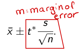
Margin of error (t - distribution)

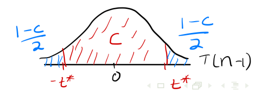
What is t*

is the upper (1 — C )/2 critical value for the T (n — 1) distribution

If the population is normal

Then ¯X is exactly normal, and so the confidence interval is exact.

If the population distribution is unknown/not normal, but the sample size is large (≥ 30)

Then ¯X is approximately normal (by the CLT), and so the confidence interval is approximate.

Example: The chief of a local police department would like to estimate the true mean response time for all emergency calls in the city. A random sample of seven emergency calls is selected, and the police response times (in minutes) are shown below:

7, 4, 11, 8, 7, 12, 9

• Construct a 95% confidence interval for the true mean response time µ of all emergency response calls in the city. Assume that response times follow a normal distribution

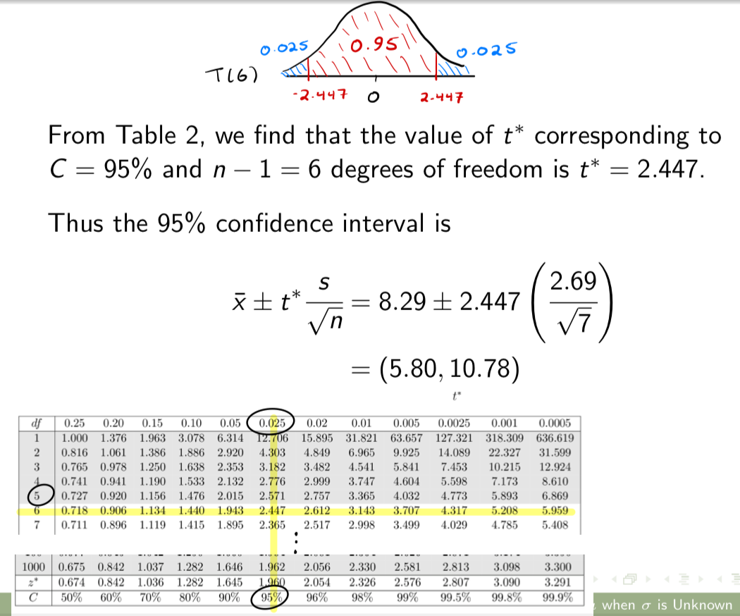
n = 7, ¯x = 8.29, s = 2.69

• From Table 2, we find that the value of t→ corresponding to C = 95% and n - 1 = 6 degrees of freedom is t* = 2.447.

• Thus the 95% confidence interval is

Example: Confidence interval

• 7, 4, 11, 8, 7, 12, 9

“If we repeatedly measured samples of seven response times in this city, and constructed intervals in a similar manner, then 95% of such intervals would contain the true mean response time µ.”

How else can we conduct hypothesis test

t distributions

Is using t distributions to conduct hypothesis different than using z

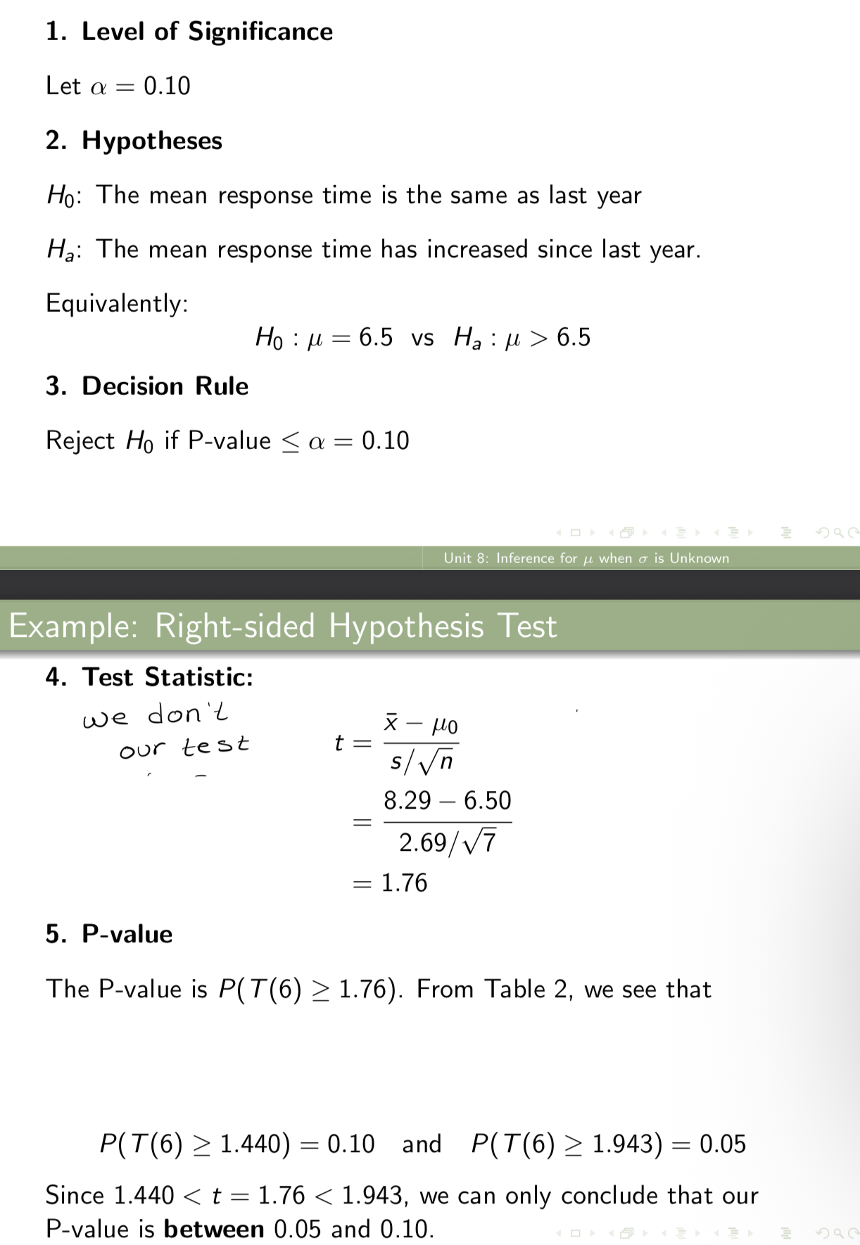
The steps of a hypothesis test using the P-value method are the same as Unit 7: the only change is that our test statistic will be t instead of z.

Example: Consider the previous example. The police chief would like to know if new measures need to be adopted in order to improve response times. Conduct a hypothesis test to determine if the mean response time has increased since the previous year, when the true mean response time was known to be 6.5 minutes. Use a significance level of 0.1

• Is this a left or right sided hypothesis test?

Right sided hypothesis test

Example: Consider the previous example. The police chief would like to know if new measures need to be adopted in order to improve response times. Conduct a hypothesis test to determine if the mean response time has increased since the previous year, when the true mean response time was known to be 6.5 minutes. Use a significance level of 0.1

Solution:

• P-value interpretation

• 6. Conclusion

P-value interpretation (The police chief would like to know if new measures need to be adopted in order to improve response times.)

“If the true mean response time was 6.5 minutes, the probability of observing a sample mean at least as high as 8.29 minutes would be between 0.05 and 0.10”

• Any value between 0.05 and 0.10 is less than or equal to α = 0.10.

• So we reject the null hypothesis!

Is it okay if the value isn’t exactly on table 2?

it is okay

Conclusion (The police chief would like to know if new measures need to be adopted in order to improve response times.)

Since the P-value ≤ α = 0.10, we reject the null hypothesis. At a 10% level of significance, we have sufficient evidence to conclude that the departments true mean response time has increased since last year.

Do I use Ζ or T?

Do I know σ?

• Yes: use Z

• No: use T

How can I tell if I know σ ?

Look for phrases like

• "the population standard deviation is ...”

• “… follow a normal distribution with standard deviation...

  • These tell you σ

How can I tell if I know s?

• "The sample standard deviation is...“

• “We take a random sample of n individuals. The standard deviation of … is calculated to be

  • Only tell us

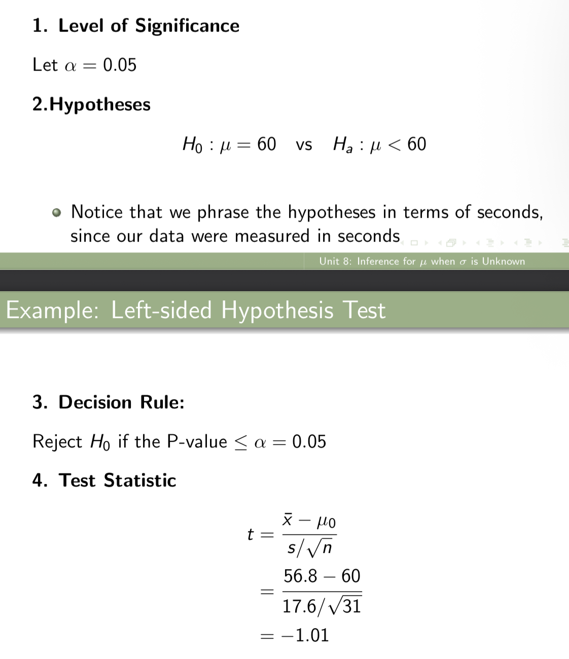
Example: A fast food restaurant claims that the average waiting time in their drive through is less than 1 minute. We record the drive through waiting times for a random sample of 31 customers. The sample average time is 56.8 seconds and the sample standard deviation is 17.6 seconds. Conduct a hypothesis test to examine the significance of the restaurant’s claim. Use a significance level of 0.05.

• Is this a left or right sided hypothesis test?

Left-sided hypothesis test

Example: A fast food restaurant claims that the average waiting time in their drive through is less than 1 minute. We record the drive through waiting times for a random sample of 31 customers. The sample average time is 56.8 seconds and the sample standard deviation is 17.6 seconds. Conduct a hypothesis test to examine the significance of the restaurant’s claim. Use a significance level of 0.05.

• solution

5. Calculation of P-value

   • interpretation of p-value

6. Conclusion

Calculation of P-value (A fast food restaurant claims that the average waiting time in their drive through is less than 1 minute.)

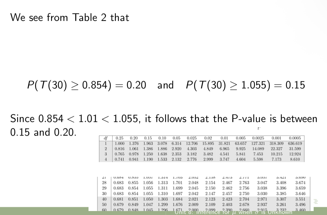
The P-value is P(T (30) ≤ -1.01) = P(T (30) ≥ 1.01) (by the symmetry of the t distribution)

• Recall that the t table uses areas to the right, not areas to the left like the z table!!!! So here, we need to rephrase our problem in terms of an area to the right

• Also notice that we had to rephrase the problem in terms of a positive t value, since there are only positive t values on Table 2

interpretation of p-value (A fast food restaurant claims that the average waiting time in their drive through is less than 1 minute.)

“If the true mean waiting time was 60 seconds, the probability of observing a sample mean at least as low as 56.8 seconds would be between 0.15 and 0.20”

• Any value between 0.15 and 0.20 is greater than α = 0.05.

Conclusion (A fast food restaurant claims that the average waiting time in their drive through is less than 1 minute.)

Since the P-value > α = 0.05, we fail to reject H0. At the 5% level of significance, we have insufficient evidence that the true mean waiting time is less than 60 seconds.

CLT

Notice that we were not told in the previous example that wait times in the drive through follow a normal distribution. This is likely not the case (in reality, wait times are likely skewed to the right)

• We had a high sample size though (≥ 30), and so by the CLT, we know the sample mean is approximately normally distributed. Thus our use of the t distribution is justified.

Example: In 2003, census results indicated that the age at which Canadian men first married had a mean of 29.7 years.

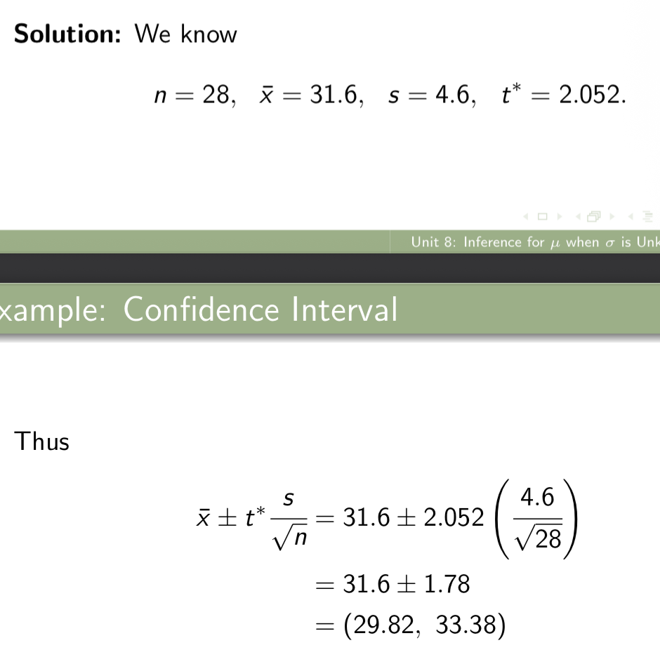
• We take a random sample of 28 men who married for the first time in 2023. Their average age is 31.6 years, and the standard deviation of their ages is 4.6 years. Assume that ages of first-time grooms are normally distributed.

1. Calculate a 95% confidence interval for the true mean age of first-time grooms in 2023

Interpretation

Interpretation of confidence interval (In 2003, census results indicated that the age at which Canadian men first married had a mean of 29.7 years.)

“If we repeatedly took samples of 28 first-time grooms and calculated intervals in a similar manner, then 95% of such intervals would contain the true mean age of all first-time grooms in 2023.”

In 2003, census results indicated that the age at which Canadian men first married had a mean of 29.7 years.

• is this a one sided or two sided hypothesis test?

two sided

Example: In 2003, census results indicated that the age at which Canadian men first married had a mean of 29.7 years.

2. Conduct a hypothesis test to determine whether the true mean age of first time grooms has changed over the last 20 years. Use α = 0.05

• p-value interpretation

• Conclusion

• Notice

P-value interpretation (In 2003, census results indicated that the age at which Canadian men first married had a mean of 29.7 years.) hypothesis test

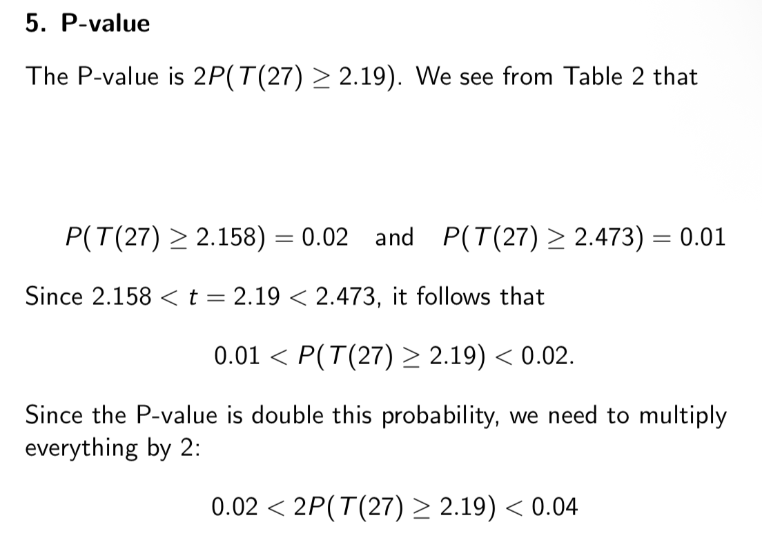
“If the true mean age of grooms has not changed over the last 20 years, the probability of observing a sample mean at least as extreme as 31.6 is between 0.02 and 0.04.”

• Any value between 0.02 and 0.04 is less than α = 0.05.

Conclusion (In 2003, census results indicated that the age at which Canadian men first married had a mean of 29.7 years.) hypothesis test

Since the P-value < α = 0.05, we reject the null hypothesis. At the 5% level of significance, we have sufficient evidence to conclude that the true mean age of first-time grooms has changed since 2003.

Notice (In 2003, census results indicated that the age at which Canadian men first married had a mean of 29.7 years.) hypothesis test

Since this is a two-sided test using a 5% level of significance, and since we already constructed a 95% confidence interval for µ, we could have used that interval to conduct the test.

• Since µ0 = 29.7 is not in the confidence interval, we reject H0.

Example: Suppose we are conducting a test of

H0 : µ= µ0 vs. Ha : µ > µ0.

• We select a sample of size 25, and we get a test statistic of t = 4.58. What is the P-value for this test?

Solution: The P-value is P(T (24) ≥ 4.58).

We see from Table 2 that P(T (24) ≥ 3.745) = 0.0005, and that 3.475 is the highest value in this row.

• Thus, since our value is even higher, we can only conclude that our P-value is less than 0.0005.

Example: Suppose we are conducting a test of

H0 : µ= µ0 vs. Ha : µ > µ0.

• We select a sample of size 16, and we get a test statistic of t = 0.53. What is the P-value for this test?

Solution: The P-value is P(T (15) ≥ 0.53)

We see from Table 2 that P(T (15) ≥ 0.691) = 0.25, and that 0.691 is the lowest value in this row.

• Thus, since our value is even lower, we can only conclude that our P-value must be greater than 0.25.

t is a function of what

function of the sample mean and of the sample standard deviation:

Is t influenced by outliers

Since both the sample mean and sample standard deviation are strongly influenced by outliers, t is also strongly influenced by outliers

What is the assumption about the population

Population is normally distributed

Is a t procedure robust against non normality

t procedures are quite robust against non-normality, especially for large sample sizes

What is the most important assumption

the data are from a SRS from the population

What additional situations will we encounter?

Data is collected in pairs

what are we interested in paired data?

Interested in the diff!erences in values of the variable for each pair, instead of in the individual observations

Paired data

means that the data have been observed in natural pairs. There are several ways in which paired data can occur:

What is measured for paired data

Two different variables are measured for each individual. We are interested in the difference between the values of the two variables

• E.g. We might be interested in the difference between an individuals STAT 1000 and STAT 2000 grade

How many times is an individual measured?

Each individual is measured twice. The two measurements of the same characteristic are made under different conditions (or at different times)

• E.g. We might measure an individuals blood pressures before and after receiving medication

How are individuals sorted?

Similar individuals are placed in pairs and each member of the pair then receives a different treatment. The same response variable is measured and compared for the two individuals in each pair

• E.g. we might place twin children on different diets, then measure the di!erence in their growth.

Why do we use matched pairs t procedures

to detect and estimate any differences between responses to two treatments

What is the parameter of interest

µd , the true mean of the differences of all pairs in the population

Can you assume that each variable follows a normal distribution

It is not enough to assume that the each variable follows a normal distribution.

What can we assume about the differences

We must assume that the

differences follow a normal distribution

What else can we assume?

that our pairs represent a SRS of all possible pairs from the population

Constructing confidence intervals and hypothesis tests in the matched pairs setting

The methods for constructing confidence intervals and hypothesis tests in the matched pairs setting are the exact same as the one-sample case

• We just have to keep in mind that we are examining differences rather than individual observations

Example: Right-sided hypothesis test

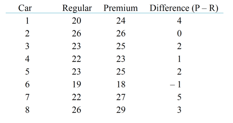
Example: Many drivers buy premium gasoline instead of regular in the belief that they will get better gas mileage. To test this belief, we obtain a sample of 8 cars. Each car is run for one tank on regular gas and one tank on premium gas, with the order randomly determined. The mileage (in miles per gallon) is measured for each car for each type of gasoline. The data are as follows:

1. Construct a 95% confidence interval for the true mean difference in mileage for premium and regular gasoline. Assume that differences d= P - R follow a normal distribution.

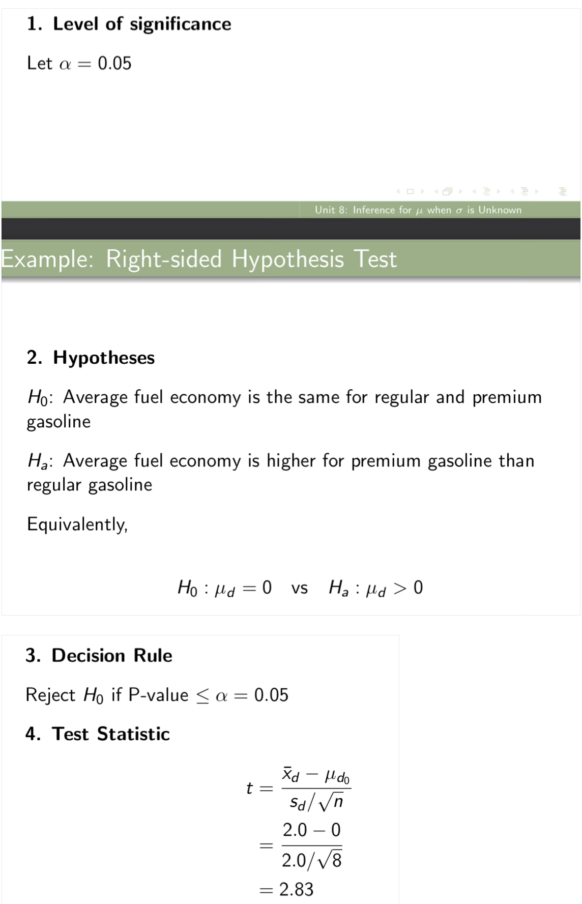
2. We would like to test whether these data provide convincing evidence that premium gasoline provides better fuel economy on average than regular gasoline. Conduct a hypothesis test with level of significance 0.05.

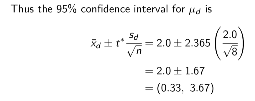
Construct a 95% confidence interval for the true mean difference in mileage for premium and regular gasoline. Assume that differences d= P - R follow a normal distribution.

(Example: Many drivers buy premium gasoline instead of regular in the belief that they will get better gas mileage.)

Solution: From the data, we calculate

n = 8,¯ xd = 2.0, sd = 2.0

• Note that the sample size n corresponds to the number of pairs in the sample.

• We also see that t* = 2.365 is the critical value from the t distribution with 7 d.f. corresponding to C = 95%.

Interpretation

Note

Interpretation (Construct a 95% confidence interval for the true mean difference in mileage for premium and regular gasoline.)

“If we took repeated samples of eight cars and calculated the interval in a similar manner, then 95% of all such intervals would contain the true mean difference in fuel economy for premium and regular gasoline”

Note (Construct a 95% confidence interval for the true mean difference in mileage for premium and regular gasoline.)

Note: it is not enough to assume that mileages for premium gas and mileages for regular gas follow normal distributions separately!!

• We must assume that the differences follow a normal distribution

Also note that for any given car, mileage for premium gas and mileage for regular gas are dependent. This means that they are related

• Notice that when two variables are dependent, this does not mean that knowing the value of one tells us the exact value of the other!

On the other hand, for any two cars, premium mileages are independent (i.e. unrelated). Similarly, for any two cars, regular mileages are independent

Notice (Construct a 95% confidence interval for the true mean difference in mileage for premium and regular gasoline.)

Notice that we could have defined the differences here the opposite way (i.e. d= R - P instead of d= P - R)

Since R - P= - (P - R), the signs of the differences would have simply switched (i.e. changed from positive to negative, or vice versa), and the interval would have been (-3.67,-0.33).

This gives us the same information, all is well!

2. We would like to test whether these data provide convincing evidence that premium gasoline provides better fuel economy on average than regular gasoline. Conduct a hypothesis test with level of significance 0.05.

Example: Many drivers buy premium gasoline instead of regular in the belief that they will get better gas mileage.

P-Value

The P-value is P(T (7) ≥ 2.83). We see from Table 2 that P(T (7) ≥ 2.517) = 0.02 and P(T(7) ≥ 2.998) = 0.01

• Since 2.517 < t = 2.83 < 2.998, the P-value is between 0.01 and 0.02.

P-interpretation

6. Conclusion

P-value interpretation (We would like to test whether these data provide convincing evidence that premium gasoline provides better fuel economy on average than regular gasoline.)

P-value is analagous to the one - sample case:

• “If there was no di!erence in average fuel economy for regular and premium gasoline, the probability of observing a sample mean difference at least as high as 2.0 mpg would be between 0.01 and 0.02”

Note that any value between 0.01 and 0.02 is less than α = 0.05

6. Conclusion: (We would like to test whether these data provide convincing evidence that premium gasoline provides better fuel economy on average than regular gasoline.)

Since the P -value < α = 0.05, we reject the null hypothesis. At the 5% level of significance, we have sufficient evidence that premium gasoline provides better fuel economy on average than regular gasoline.

• If we had instead defined the di!erences as d= R - P, then:

  • the value of the test statistic would have been t = -2.83 and

• the P -value would have been P(T (7) ≤ -2.83), which is the same as the P-value we calculated.

• Thus the conclusion would be the same

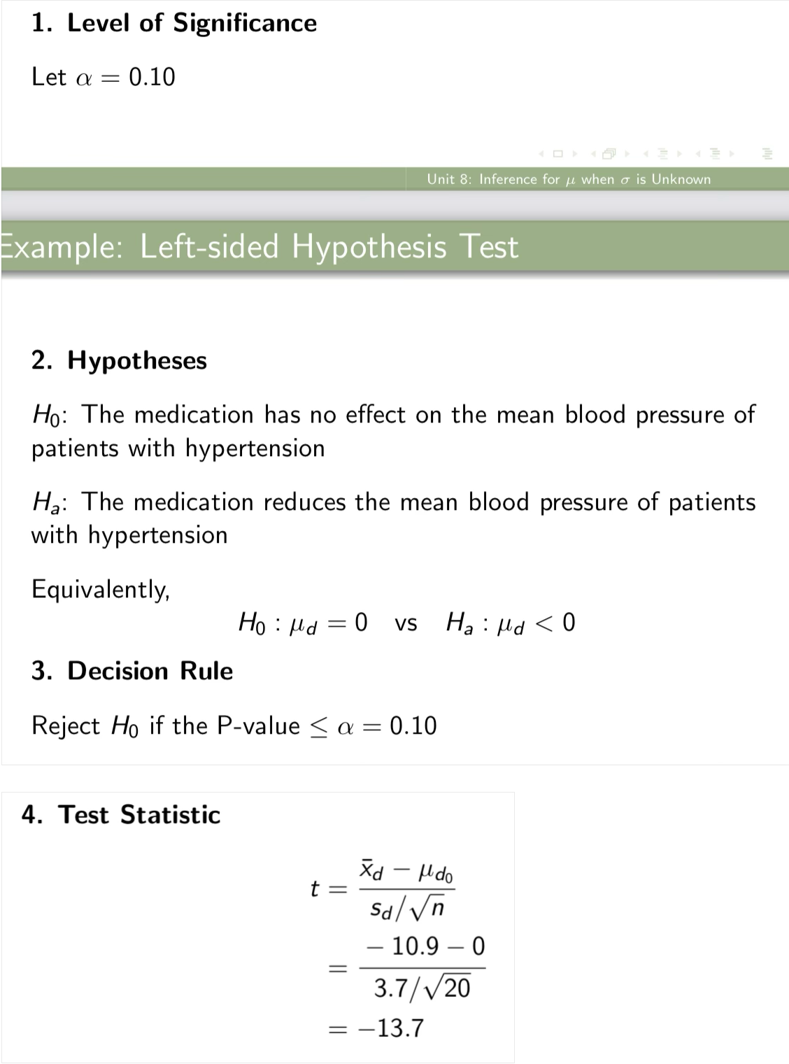
Example: Left-sided hypothesis test

Example: A pharmaceutical company is testing a new blood pressure medication. The systolic blood pressures of a sample of 20 patients with hypertension are measured before and after taking the medication, and we calculate the di!erences d = After - Before. We calculate the sample mean di!erence to be ¯ xd = -10.9 and the sample standard deviation of the differences to be sd = 3.7.

• Conduct a hypothesis test to determine whether the medication is successful in reducing systolic blood pressure with α = 0.10. Assume that the di!erences follow a normal distribution.

5. Calculation of P-value

• The P-value is P(T (19) ≤ -13.7) = P(T (19) ≥ 13.7) (by the symmetry of the t distributions).

• We see from Table 2 that P(T (19) ≥ 3.883) = 0.0005

Since 13.17 > 3.883, the P-value is less than 0.0005.

P-value interpretation

6. Conclusion

Notice

P-value interpretation (A pharmaceutical company is testing a new blood pressure medication.)

If there was no difference in average blood pressure before and after taking the medication, the probability of observing a sample mean difference at least as low as -10.9 would be less than 0.0005.”

• Any value less than 0.0005 is less than α = 0.10.

6. Conclusion (A pharmaceutical company is testing a new blood pressure medication.)

Since the P-value < α = 0.10, we reject the null hypothesis. At the 10% level of significance, we have sufficient evidence that the medication reduces the mean blood pressure of patients with hypertension.

Notice (A pharmaceutical company is testing a new blood pressure medication.)

• In this example, notice that for any given patient, blood pressure before and after taking the medication are dependent

• On other hand, for any two patients, the blood pressure before (or after) are independent

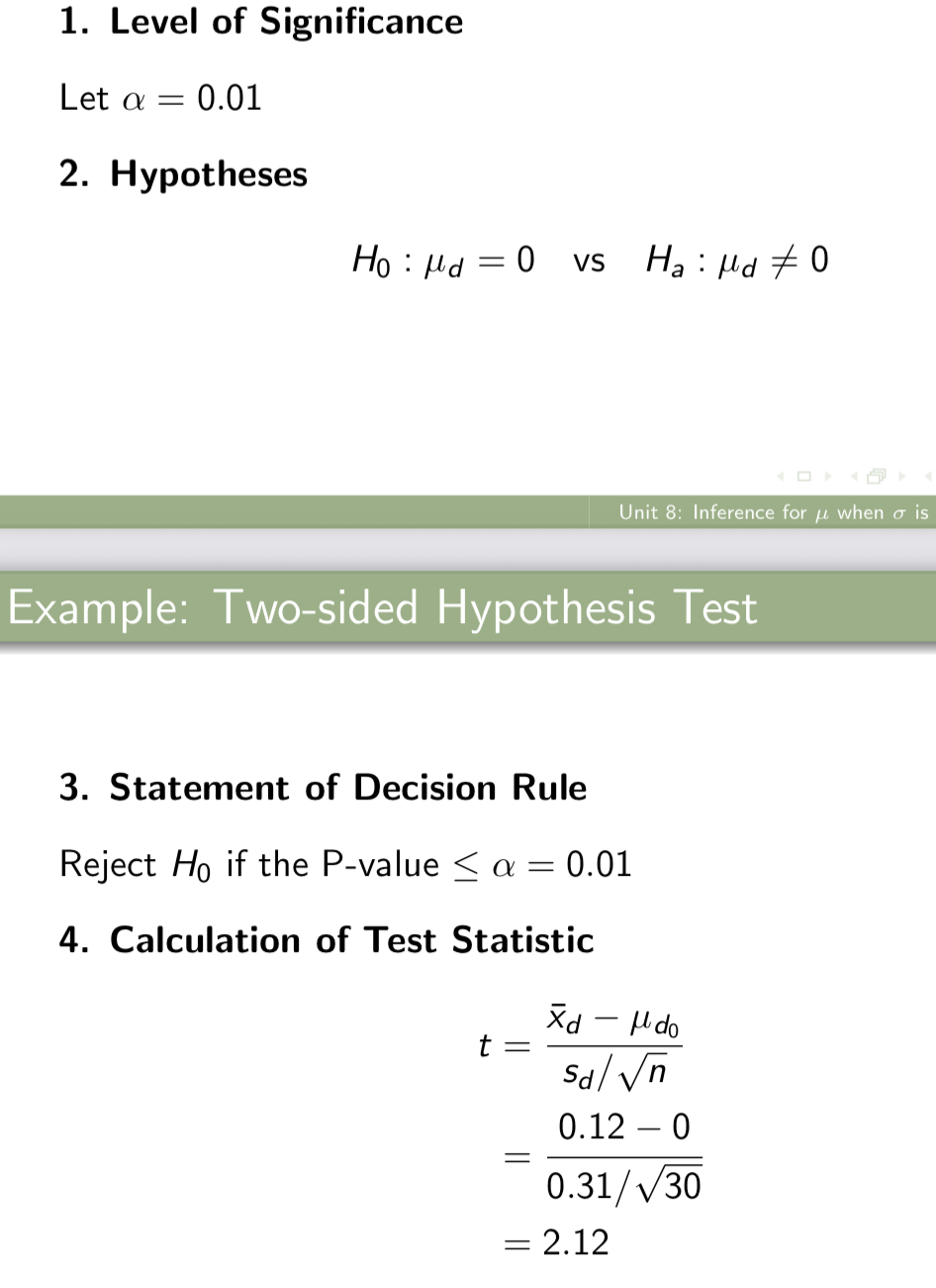
Example: Many psychology studies have examined the di!erences between the first and second children in a family. Suppose we would like to compare their academic performance. We examine the high school GPAs of a sample of 30 pairs of siblings and calculate the difference in GPAs, d = first child - second child. We calculate an average difference of ¯ xd = 0.12 and a standard deviation of sd = 0.31. Assume that differences follow a normal distribution .

1. Calculate a 99% confidence interval for the true mean difference in GPAs.

2. Conduct a hypothesis test to determine whether there is evidence of a difference in the average high school academic performance between the first and second children in a family. Use α = 0.01.

example of confidence interval

1. Calculate a 99% confidence interval for the true mean difference in GPAs.

Solution: We know

¯xd = 0.12, sd = 0.31, n = 30, t* = 2.756

• Here, t* is the critical value from the t distribution with 29 d.f. for C = 99%

Confidence interval interpretation

confidence interval interpretation (99% confidence interval for the true mean difference in GPAs.)

“If we took repeated samples of 30 pairs of siblings and calculated the interval in a similar manner, 99% of such intervals would contain the true mean di!erence in high school GPAs for the first and second children in a family.”

• Notice that for any pair of siblings, high school GPAs are dependent

Two - sided hypothesis test

2. Conduct a hypothesis test to determine whether there is evidence of a difference in the average high school academic performance between the first and second children in a family. Useε = 0.01.

5. Calculation of P-value

• The P-value is 2P(T (29) ≥ 2.12). We see from Table 2 that

  • P(T (29) ≥ 2.045) = 0.025 and P(T (29) ≥ 2.150) = 0.02

• Since 2.045 < t = 2.12 < 2.150, we know P(T (29) ≥ 2.12) is between 0.02 and 0.025.

• Since the P-value is 2P(T (29) ≥ 2.12), it follows that the P-value is between 2(0.02) = 0.04 and 2(0.025) = 0.05.

P-value interpretation

Conclusion

Note

Also note

P-value interpretation (Two - sided hypothesis test - high school academic performance between the first and second children in a family.)

If there was no difference in average high school academic performance for first and second children, the probability of observing a sample mean difference at least as extreme as 0.12 is between 0.04 and 0.05.”

• Any value between 0.04 and 0.05 is greater than α = 0.01

Conclusion (Two - sided hypothesis test - high school academic performance between the first and second children in a family.)

Since the P -value > α = 0.01, we fail to reject the null hypothesis. At the 1% level of significance, we have insufficient evidence that there is a difference in average high school academic performance between the first and second children in a family.

Note (Two - sided hypothesis test - high school academic performance between the first and second children in a family.)

• If we had defined the difference as d = second child - first child, the value of the test statistic would have been t = -2.12 and the P -value would have been 2P(T (29) ≤ -2.12)

• This is the same as the P-value we calculated. So the conclusion would have been the same.

Also note (Two - sided hypothesis test - high school academic performance between the first and second children in a family.)

Since this was a two-sided test with a 1% level of significance, we could have used the 99% confidence interval to conduct the test

• We calculated previously that the 99% confidence interval for µd is (-0.036, 0.276)

• Since µd0 = 0 is contained in the 99% confidence interval for µd , we fail to reject H0 at the 1% level of significance.