BMM Module 8: Molecular Dynamics

What is MD

computer simulations that allow us to study atoms and molecules and their interaciton over a period of time using known laws of physics (newtonion)
example: study how cholesterol inserts into the membrane

why do we need MD?

• bridge theory and experiment:

  • practical model when experiments are too expensive or difficult

  • But simulations are hard to prove to be correct

• Capture atomic motions or interactions that cannot be observed in the lab

• Fills the gap where other measurements fall short like NMR or FRET

• examples

  • local/global conformations

  • enzyme substrate binding

  • free energy determination

  • protein folding

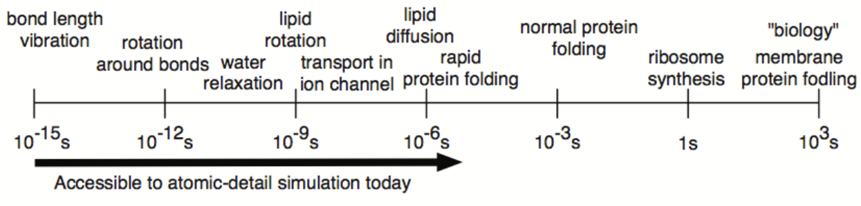
today MD simulations typically range from a 100’s of ns to a few µs

(normal protien folding is however in the range of ms)

How does MD work?

The force field determines the energy of the system: bonded + non bonded interactions

Non bonded interactions combine attraction and repulsion and therefore cause the biggest movement

E_VDW : use a neighbour list

• every atom keeps a list of nearby atoms within a certain cut off distance (9-12A)

• the list is updated every few steps because atoms move during the simulations

• only these atoms are considered for interactions which reduces computational cost

E_{electrostatic}

• need to account for the surrounding medium

  • permitivity tells you strongly charges are screened compared to vacuum

• No NB lis is used: electrostatic interactions don’t decay as rappid

• Solution: PME = Particle Mesh Ewald Summation

  • mesh of charges constructed to treat long range interactions

Solvent representations in MD

Explicit water model

• treat every water molecule as an individual entity (with physical properties) within the simulation box

Implicit water model

• treat water as a continuous background medium= average effect of water

• faster but less accurate

computational power is now big enough to mostly use the explicit water model

Steps in MD: 1-3

1. add H’s using GROMACS (MD simulation package)

   1. not in X-ray crystal structures because to low electron density

2. Put the protein into a simulation box = unit cell

   1. computer needs a finite folume to compute interactions and motions

   2. infinite space would be unrealistic and computationally impossible to handle

   3. usually cubic or triclinic

   4. better= rhombic decahedron or truncated octahedron which are smaller than cubic and thus incorporate less water far away from the protein that would need to be computed

3. PBC = period boundry conditions = copy cell in all directions

   1. this is done to mimmic large solvent environment rather than a tiny droplet

   2. This eliminates edge artifacts, particles at the edge would be in contact with vaccuum leading to surface tension errors

   3. Mainting a constant particle density: for particles leaving at one edge, an identical copy would enter from the other side

Steps in MD: 4-5

4. Determine the box size

   1. it sould be bigger than the non bonded cut off (9-12A)- but not to large (extra water)

   2. this avoids proteins from interacting or that water molecules in between are attracted by both

5. Add solvent

   1. Algorithm randomly adds water molecules in a way that agrees with the density of water

   2. Counter ions are added to screen charges and neutralise the system (without charges would accumulate and charges in boxes will repel)

      1. not OH^- or H⁺ because these would alter the pH

   3. Energy minimize to remove steric clashes and relax the solvent

Steps in MD: 6

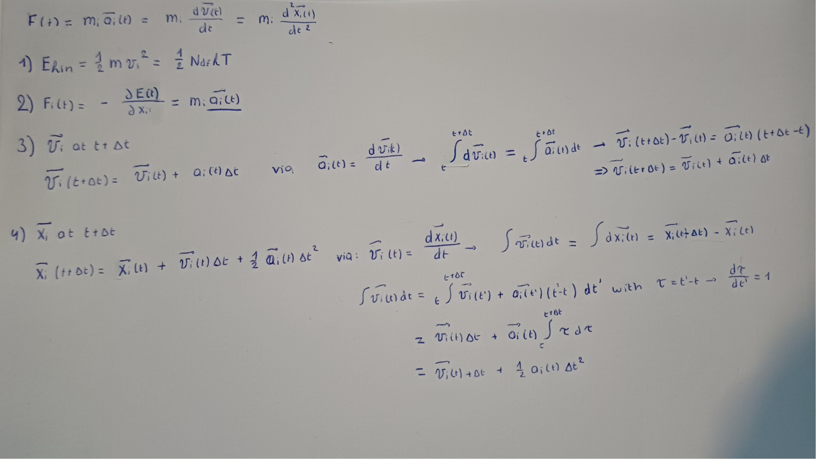
Start dynamics according to Newtons laws of motion

Essence of MD: if we know the force acting on all atoms we can calculate the a, v and x over time

1. assign each atom an initial velocity based on th gaussian distribution at a certain T

   1. give us the kinetic energy

2. Calculate the force on each atom

   1. derivative of the energy, an can be used to calculate acceleration

3. calculate the speed at the next step

   1. from a and t

4. calculate the postion at the next step

   1. from v_i , a_i and t

5. Energies and coordinates are written to trajectory files

6. repeating this process generates the MD trajectory

• the time step is usually 2 fs = 2 ×10^-15 s

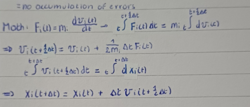
leap frog scheme

method that doesn’t try to find position and velocity at the same time but instead ofsets them by half a timestep

1. calc the velocity at t+1/2Δt

2. use that to calculate the xi at a full time step ( t+Δt)

3. use that to jump velocity to the next half step

This creates a balance were errors in first step are often cancelled by the second step - so no accumulation of errors

NVE

The system we’ve now created contains a constant amount of particle (N), cte Volume (V) and constant E = microcanonical ensemble

The total energy is converved
E = Ekin+Epot
particle can move freely constantly exchanging kinetic and potential energy

For our simulation to match conditions of an experiment, we need to swithc our ensemble (most experiments are conducted at constant energy pressure, not energy and volume)

• NVE—> NVT: thermostat alters particle velocity so average Ekin corresponds to the target temperature

  • so system can exhange E with heat bath and E is no longer conserved

• NVT —> NVP (barostat) alter the size of the box dynamically so average pressure matches the target value

switching to NVT and NVP ensure the system can reach and remain at thermal equilibrium and reach a physically realistic density

How this fits in an MD workflow

1. System setup (before simulation)

Before any dynamics:

• Build the system (structure, box, solvent, ions)

• Assign force-field parameters

• Choose initial positions and initial velocities

At this point, no ensemble is “running” yet — you just define initial conditions.

2. Equilibration phase

Once the simulation starts:

a) Start in NVE

• Initial velocities define the total energy

• Particles move according to Newton’s equations

• Energy is (ideally) conserved

This step is often very short or implicit, mainly to check stability.

b) Switch to NVT

• A thermostat is applied

• Particle velocities are adjusted so the average kinetic energy matches the target temperature

• The system exchanges energy with a heat bath

• Total energy is no longer conserved

Purpose: bring the system to the correct temperature

c) Switch to NPT

• A barostat is added

• The simulation box size changes dynamically

• The system reaches the correct average pressure and density

Purpose: obtain a physically realistic density

3. Production run (after equilibration)

After equilibration:

• You typically run long simulations in:

  • NPT (to mimic experimental conditions),

GROMACS

= MD package that can genereate trajectoreis which record how atom positions, velocities and forces change over time

• this can be used to calculate how structural and dynamic poperties evolve over time

• this is where analysis begins

  • e.g. RMSD of a ligand in a binding pocket over time

trajectory vs topology

trajectory describes how thing move

topology contains fixed atom info

How can we use MD

1. dowload proteins from PDB or use homology model if structure is unknown

   1. carefully investigate input structure: garbe in= garbe out

   2. Also use sufficient heating to explore many conformations on the PES

2. Run MD simulation

3. Analysis

   1. RMSD = how protien changes conformation over time from starting point

   2. RMSF = root mean square fluctuation = describe how each atom/ residue in a molecule fluctuates around its average position over time

   3. R_G : radius of gyration = how does the molecule change shape

   4. PCA = principle component analysis
      Reduces dataset to a small number of principle components with new axes capturing the most important motions an variations in the system
      Each PC represents:

      1. direction along which atoms move together

      2. eigenvalue: how much motion there is along that direction

applications of MD

• conformational changes
  analyze physical process of the HIV-1 fusion peptide changes conformation when interacting with the host cell membrane

• protein ligand binding
  see how interactions evolve, how stable they are, how water and protein flexibility influence binding

• protein folding

  • only small proteins (µs)

  • why? correct foldingis essential for function of a protein, misfolding present many diseases

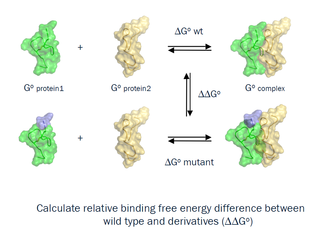
• binding free energy calculation