ECON Maths pt 2

Define limit of a function due to Heine

Given the function f: A⊂R^N→R, a∈R is a limit of f(x) as x→x0∈A if

∀{x_n}∈A: lim_(n→∞)x_n=x₀∈A ⟹ f(x_n)→a

Define limit of a function due to Cauchy

Given the function f:A⊂RN→R, a∈R is a limit of f(x) as x→x0∈A if

∀ϵ>0, ∃δ>0 such that 0<|x−x₀|<δ⟹|f(x)−a|<ϵ

• note the similarity to the definition of the sequence

• note that in the ϵ-ball around x0 the point x0 is excluded

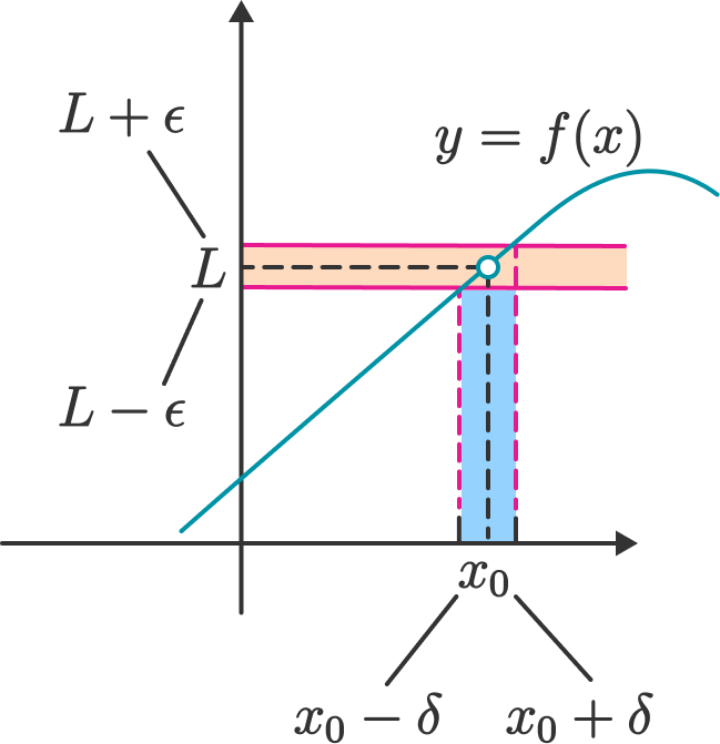
Fig. 45 limx→x₀f(x)=L under the Cauchy definition#
Fact: Cauchy and Heine definitions of the function limit are equivalent

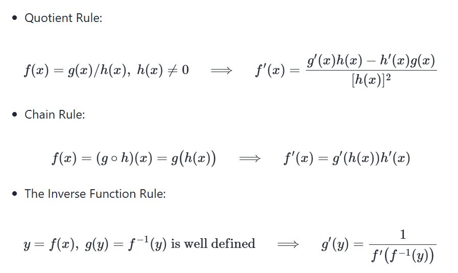
quotient / inverse function rules

differentiability relationship with continuity

Differentiability ⟹ Continuity

Differentiability ⟸̸ Continuity

Little-o

Little-o notation is used to describe functions that approach zero faster than a given function

f(x)=o(g(x)) as x → a ⟺ lim_(x→a)f(x)g(x)=0

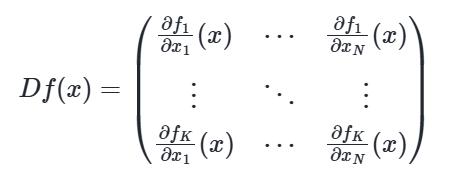
Define total derivative (Jacobian)

If a vector-valued function f: R^N→R^K is differentiable at x, then all partial derivatives at x exist and the (_) is given by

(matrix - see image)

Note:

• note that partial derivatives of a vector-valued function f are indexed with two subscripts: i for f and j for x

• index i∈{1,…,K} indexes functions and rows of the Jacobian matrix

• index j∈{1,…,N} indexes variables and columns of the Jacobian matrix

• Jacobian matrix is (K×N), i.e. number of functions in the tuple by the number of variables

• the gradient is a special case of Jacobian with K=1, as expected!

Sufficient conditions for differentiability of a function f: R^N→R^K at x are that all partial derivatives exist and are continuous in x

Rules of differentiation multivariate calculus - Sum and scaling

Let A denote an open set in RN and let f,g: A→R^K be differentiable functions at x∈A.

1. f+g is differentiable at x and D(f+g)(x)=Df(x)+Dg(x)

2. cf is differentiable at x and D(cf)(x)=cDf(x) for any scalar c

Define outer product

Outer product of two vectors x∈RN and y∈RK is a N×K matrix given by

xy′=(x1⋮xN)(y1,…,yK)=(x1y1⋯x1yK⋮⋱⋮xNy1⋯xNyK)

Note: Potential confusion with products continues: in current context scalar product is a multiplication with a scalar (and not the product that produces a scalar as before in dot product of vectors)

Dot product rule

Fact: Dot product rule

Let A denote an open set in RN and let f,g:A→R^K be both differentiable functions at x∈A. Assume that both functions output column vectors.

Then the dot product function f⋅g:A→R is differentiable at x and

∇(f⋅g)(x) = f(x)^TDg(x)+g(x)^TDf(x),

where ◻^T denotes transposition of a vector.

Observe that:

• both Dg(x) and Df(x) are (K×N) matrices

• both f(x)T and g(x)T are (1×K) row-vectors

• therefore, both f(x)TDg(x) and g(x)TDf(x) are (1×N) row-vectors

Chain rule

Fact: Chain rule

Let

• A denote an open set in R^N

• B denote an open set in R^K

• f: A→B be differentiable at x∈A

• g: B→R^L be differentiable at f(x)∈C

Then the composition g∘f is differentiable at x and its Jacobian is given by

D(g∘f)(x)=Dg(f(x))Df(x)

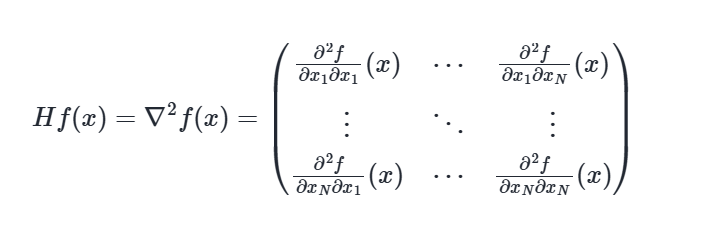
Define Hessian

Let A denote an open set in R^N, and let f:A→R. Assume that f is twice differentiable at x∈A.

The total derivative of the gradient of function f at point x, ∇f(x) is called the (_) matrix of f denoted by Hf or ∇2f, and is given by a N×N matrix

State Young’s Theorem

Fact (Young’s theorem)

For every x∈A ⊂ R^N where A is an open and f:A→R^N is twice continuously differentiable, the Hessian matrix ∇2f(x) is symmetric

State the Clairaut Theorem

Fact (Clairaut theorem)

If all the k-th order partial derivatives of f exist and are continuous in a neighbourhood of x, then the order of differentiation does not matter, and the mixed partial derivatives are equal

Define and state properties of dot product

The dot product of two vectors x,y∈R^N is

x⋅y=x^Ty=∑^N_n=1x_ny_n

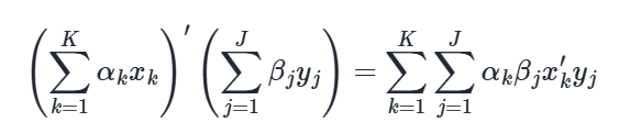
Fact: Properties of dot product

For any α,β∈R and any x,y∈R^N, the following statements are true:

1. x^Ty=y^Tx

2. (αx)′(βy)=αβ(x^Ty)

3. x^T(y+z)=x^Ty+x^Tz

Define the (Euclidean) norm

The (_) (_) of x∈R^N is defined as

‖x‖=sqrt(x^Tx)=(∑^N_n=1x²_n)^1/2

• ‖x‖ represents the ``length’’ of x

• ‖x−y‖ represents distance between x and y

linear algebra - inequalities

For any α∈R and any x,y∈R^N, the following statements are true:

1. ‖x‖≥0 and ‖x‖=0 if and only if x=0

• ‖αx‖=|α|‖x‖

• ‖x+y‖≤‖x‖+‖y‖ (triangle inequality)

• |x^Ty|≤‖x‖‖y‖ (Cauchy-Schwarz inequality)

Linear combinations

Definition

A linear combination of vectors x₁,…,x_K in R^N is a vector

y=∑^K_k=1 α_kx_k = α₁x₁+⋯+α_Kx_K

where α1,…,αK are scalars

Inner products of linear combinations satisfy

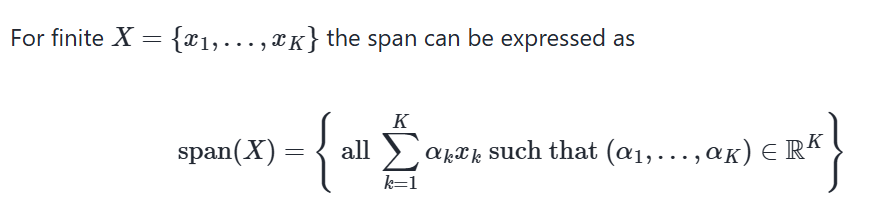
Define span

Set of all possible linear combinations of elements of X is called the (_) of X, denoted by span(X)

Define linear subspace (subspace)

A nonempty S⊂R^N called a linear subspace of R^N if

x, y ∈ S and α, β ∈ R ⟹ αx + βy∈ S

In other words, S⊂R^N is “closed” under vector addition and scalar multiplication

canonical

The set of canonical basis vectors {e₁,…,e_N} is linearly independent in R^N

linearly independent

Fact

Take X={x₁,…,x_K}⊂R^N. For K>1 all of following statements are equivalent

1. X is linearly independent

2. No x_i ∈ X can be written as linear combination of the others

3. X₀ ⊂ X ⟹ span(X₀) ⊂ span(X)

Facts of linear independence (4)

Fact If X is linearly independent, then X does not contain 0

Fact If X is linearly independent, then every subset of X is linearly independent

Fact If X={x₁,…,x_K} ⊂ R^N is linearly independent and z is an N-vector not in span(X), then X∪{z} is linearly independent

Fact If X={x₁,…,x_K} ⊂ R^N is linearly independent and y ∈ R^N, then there is at most one set of scalars α₁,…,α_K such that y=∑^K_k=1 α_kx_k

Exchange Lemma

Let S be a linear subspace of R^N, and be spanned by K vectors.
Then any linearly independent subset of S has at most K vectors

Define the basis

Let S be a linear subspace of R^N

A set of vectors B={b1,…,bK} ⊂ S is called a basis of S if

1. B is linearly independent

2. span(B)=S

e.g. Canonical basis vectors form a basis of R^N

Define linear function

A function T:RK→RN is called (_) if

T(αx+βy)=αTx+βTy∀x, y∈R^K, ∀ α, β ∈ R

Define the null space (kernel)

The (_) or (_) of linear mapping T:R^K→R^N is

kernel (T)={x∈R^K:Tx=0}

If T is a linear function from R^N to R^N then all of the following are equivalent:

If T is a linear function from R^N to R^N then all of the following are equivalent:

1. T is a bijection

2. T is onto/surjective

3. T is one-to-one/injective

4. kernel(T)={0}

5. The set of vectors V={Te₁,…,Te_N} is linearly independent

Definition: If any one of the above equivalent conditions is true, then T is called nonsingular

Fact: If T:R^N→R^N is nonsingular then so is T⁻¹

For a linear mapping T from R^K→R^N, the following statements are true:

1. If K<N then T is not onto

2. If K>N then T is not one-to-one

Define Rank

The dimension of span(A) is known as the (_) of A

rank(A)=dim(span(A))

Because span(A) is the span of K vectors, we have

rank(A) = dim(span(A))≤K

Definition

A is said to have full column rank if

rank(A)= number of columns of A

Define nonsingular for square matrix A

We say that A is nonsingular if T: x→Ax is nonsingular

Equivalent:

• x↦Ax is a bijection from RN to RN

We now list equivalent conditions for nonsingularity

Fact Let A be an N×N matrix
All of the following conditions are equivalent

1. A is nonsingular

2. The columns of A are linearly independent

3. rank(A) = N

4. span(A) = R^N

5. If Ax=Ay, then x=y

6. If Ax=0, then x=0

7. For each b ∈ R^N, the equation Ax=b has a solution

8. For each b ∈ R^N, the equation Ax=b has a unique solution

Define invertible

Given square matrix A, suppose ∃ square matrix B such that

AB=BA=I

Then

• B is called the inverse of A, and written A⁻¹

• A is called invertible

Fact A square matrix A is non-singular if and only if it is invertible

State the inverse of a 2×2 matrix

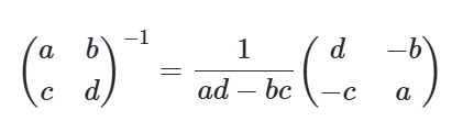
Define
a) eigenvalue
b) eigenvector
c) eigenpair

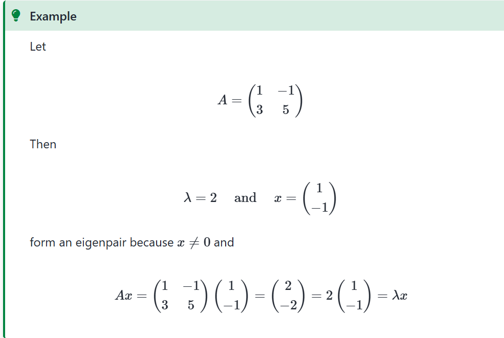
Let A be a square matrix

Think of A as representing a mapping x↦Ax, (this is a linear function)

But sometimes x will only be scaled:

Ax=λx for some scalar λ

Definition

If Ax=λx holds and x is nonzero, then

1. x is called an (_b_) of A and λ is called an (_a_)

2. (x,λ) is called an (_c_)

Eigenvalues and determinants

For any square matrix A

λ is an eigenvalue of A ⟺ det(A−λI) = 0

Define
a) characteristic polynomial
b) characteristic equation

The polynomial det(A−λI) is called a (_a_) of A.

The roots of the (_b_) det(A−λI)=0 determine all eigenvalues of A.

Define similar (matrix)

Square matrix A is said to be (_) to square matrix B if there exist an invertible matrix P such that A=PBP⁻¹.

If the linear map is the same, we must have

Ax=PBP⁻¹x

Fact

Given N×N matrix A with distinct eigenvalues λ1,…,λN we have

• If A=diag(d1,…,dN), then λn=dn for all n

• det(A)=∏n=1Nλn

• If A is symmetric, then λn∈R for all n (not complex!)

Proof

Fact A is nonsingular ⟺ all eigenvalues are nonzero

Fact If A is nonsingular, then eigenvalues of A⁻¹ are 1/λ₁,…,1/λ_N

Conic sections

An equation describing every conic section is a quadratic equation in two variables.

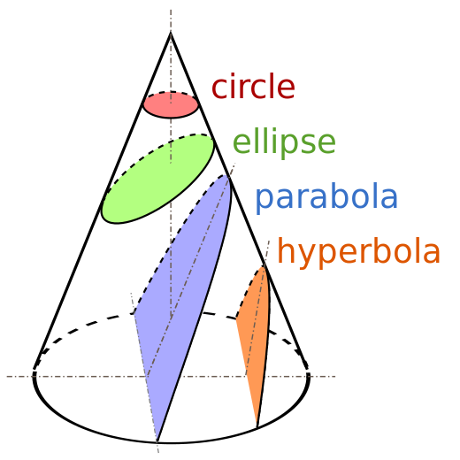
Fig. 68 Conic sections#

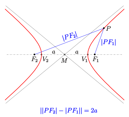
Define Hyperbola

(_) is a collection of points (x,y) ∈ R², the difference of distances from which to two fixed points (termed foci) is constant.

Define Quadratic form

(_) form in a function Q:R^N→R

Q(x)=∑^N_i=1∑^N_j=1a_ijx_ix_j

(_) form Q:R^N→R can be equivalently represented as a matrix product

Q(x)=x^TAx

where x∈R^N is a column vector, and (N×N) symmetric matrix A consists of elements {a_ij}, i,j=1,…,N

Changing bases

Fact By change of bases any quadratic form Q(x) with a symmetric real matrix A can be transformed to a sum of squares with positive or negative coefficients

Q(x)=x^TAx = x^TP^TDPx =(Px)^TD(Px)=∑^N_i=1λ_i(Px)²_i

where λ_i are the eigenvalues and P is the matrix of eigenvectors of A.

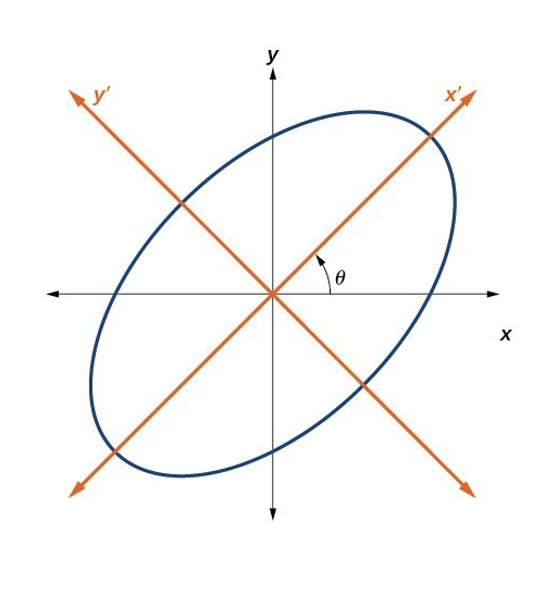
Fig. 69 Change of bases to convert the quadratic form to a canonical form

Define
a) positive definite
b) negative definite

Quadratic form Q(x) is called (_a_) if

Q(x)=x^TAx>0 for all x≠0

Quadratic form Q(x) is called (_b_) if

Q(x)=x^TAx<0 for all x≠0

• the examples above show these cases

• note that because every quadratic form can be represented by a linear combination of squares, the characteristic properties are the signs of the coefficients in the canonical form!

Law of inertia

Fact (law_)

The number of coefficients of a given sign in the canonical form of a quadratic form does not depend on the choice of the basis

Define Definite

Positive and negative definite quadratic forms are called (_)

Note that for some matrices it may be that

• for some x: x^TAx < 0

• for some x: x^TAx > 0

In this case A is called indefinite

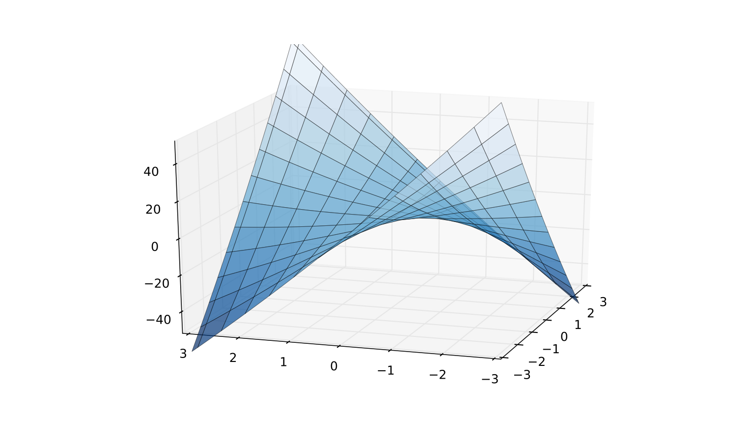
Fig. 72 Indefinite quadratic function

Q(z)= x²₁ /2+8x₁x₂+x²₂ /2

Define positive semi-definite (aka. non-negative definite)

Quadratic form Q(x) is called non-negative definite (positive semi-definite) if

Q(x)=x^TAx⩾0 for all x≠0

Quadratic form Q(x) is called non-positive definite (negative semi-definite) if

Q(x)=x^TAx⩽0 for all x≠0

Facts definite(ness)

Fact: If quadratic form x^TAx is positive definite, then det

Fact (definiteness)

Let A be an (N×N) symmetric square matrix. The corresponding quadratic form Q(x)=xTAx is positive definite if and only if all leading principal minors of A are positive

x^TAx>0 for all x≠0⟺M_k>0 for all k=1,…,N

Quadratic form Q(x)=x^TAx is negative definite if and only if the leading principal minors of A alternate in sign according to the following rule

x^TAx<0 for all x≠0⟺(−1)^kM_k>0 for all k=1,…,N

Fact (semi-definiteness)

Fact (semi-definiteness)

Let A be an (N×N) symmetric square matrix. The corresponding quadratic form Q(x)=x^TAx is positive semi-definite if and only if all principal minors of A are non-negative.

x^TAx⩾0 for all x≠0⟺∀P_k:P_k⩾0 for all k=1,…,N

Quadratic form Q(x)=x^TAx is negative semi-definite if and only if all principal minors of oder k of A are zero or have the same sign as (−1)^k

x^TAx⩽0 for all x≠0⟺∀P_k:(−1)^kP_k⩾0 for all k=1,…,N

Components of the optimization problem

1. Objective function: function to be maximized or minimized, also known as maximand
   In the example above profit function π(p,q)=pq−C(q) to be maximized

2. Decision/choice variables: the variables that the agent can control in order to optimize the objective function, also known as controls
   In the example above price p and quantity q variables that the firm can choose to maximize its profit

3. Equality constraints: restrictions on the choice variables in the form of equalities
   In the example above q=α+14αp2−p

4. Inequality constraints (weak and strict): restrictions on the choice variables in the form of inequalities
   In the example above q≥0 and p>0

5. Parameters: the variables that are not controlled by the agent, but affect the objective function and/or constraints
   In the example above α, β and δ are parameters of the problem

6. Value function: the “optimized” value of the objective function as a function of parameters
   In the example above Π(α,β,δ) is the value function

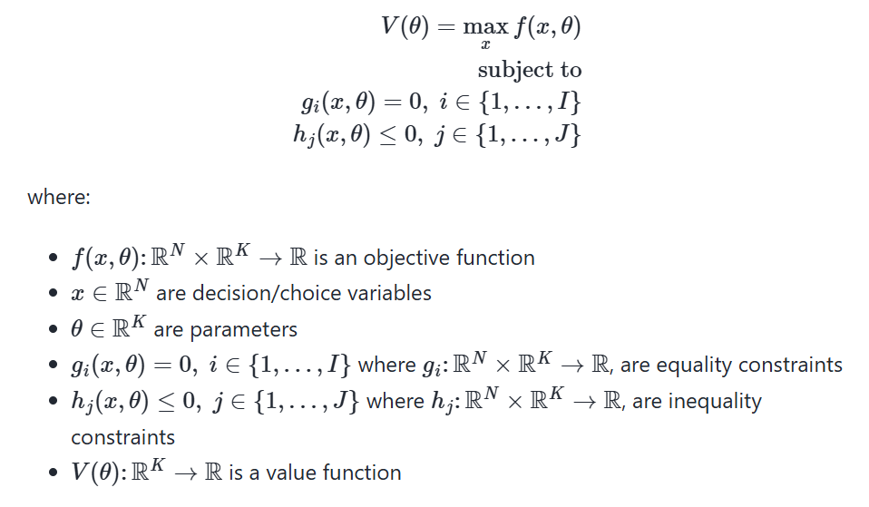
Define the general form of the optimisation problem

The (_) is

V(θ)=max_(x) f(x,θ) subject to g_i(x,θ)=0, i∈{1,…,I}hj(x,θ)≤0, j∈ {1,…,J}

where:

• f(x,θ): R^N×R^K→R is an objective function

• x∈R^N are decision/choice variables

• θ∈R^K are parameters

• g_i(x,θ)=0,i ∈ {1,…,I} where g_i: R^N×R^K→R, are equality constraints

• h_j(x,θ)≤0, j∈{1,…,J} where h_j: R^N×R^K→R, are inequality constraints

• V(θ):R^K→R is a value function

Define the set of admissible choices (admissible set)

The set of (_) contains all the choices that satisfy the constraints of the optimization problem.

Reminder of definitions

A point x∗∈[a,b] is called a

• maximizer of f on [a,b] if f(x∗)≥f(x) for all x∈[a,b]

• minimizer of f on [a,b] if f(x∗)≤f(x) for all x∈[a,b]

Point x is called interior to [a,b] if a<x<b

A stationary point of f on [a,b] is an interior point x with f′(x)=0

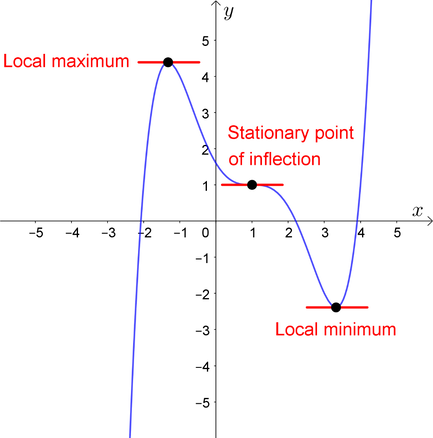
Fig. 73 Both x∗ and x∗∗ are stationary

Define stationary point

Definition

Given a function f: R^N→R, a point x∈R^N is called a stationary point of f if ∇f(x)=0

Definition

Given a function f: R^N → R, a point x*∈R^N is called a local maximiser/minimiser of f if ∃ϵ such that f(x)≤ f(x*) for all x∈Bϵ(x*)

If the inequality is strict, then x* is called a strict local maximiser/minimiser of f

A maximiser/minimiser (global) must also be a local one, but the opposite is not necessarily true.

State the necessary condition for optima

Let f(x,θ): R^N→R be a differentiable function and let x*∈ R^N be a local maximiser/minimiser of f.

Then x* is a stationary point of f, that is ∇f(x*)=0

saddle point

• saddle point where the FOC hold, yet the point is not a local maximizer/minimizer!

• Similar to x=0 in f(x)=x3: derivative is zero, yet the point is not an optimizer

• How to distinguish saddle points from optima? Key insight: the function has different second order derivatives in different directions!

• need SOC to distinguish

SOC

• do not give definitive answer in all cases, unfortunately

Fact (necessary SOC)

Let f(x): R^N→R be a twice continuously differentiable function and let x*∈ R^N be a local maximiser/minimiser of f. Then:

• f has a local maximum at x*⟹Hf(x*) is negative semi-definite

• f has a local minimum at x*⟹Hf(x*) is positive semi-definite

• recall the definition of semi-definiteness

Fact (sufficient SOC)

Let f(x): R^N→R be a twice continuously differentiable function. Then:

• if for some x*∈ R^N ∇f(x*)=0 (FOC satisfied) and Hf(x*) is negative definite, then x* is a strict local maximum of f

• if for some x*∈R^N ∇f(x*)=0 (FOC satisfied) and Hf(x*) is positive definite, then x* is a strict local minimum of f

• observe that SOC are only necessary in the “weak” form, but are sufficient in the “strong” form

• this leaves room for ambiguity when we can not arrive at a conclusion — particular stationary point may be a local maximum or minimum

• but we can rule out saddle points for sure, in this case neither semi-definiteness nor definiteness can be established, the Hessian is indefinite

SOC provide:

Fact Given a twice continuously differentiable function f: R² → R and a stationary point x*: ∇f(x*)=0, the second order conditions provide:

1. if det(Hf(x*))>0 and trace(Hf(x*))>0 ⟹

   • λ₁>0 and λ₂>0,

   • Hf(x*) is positive definite,

   • f has a strict local minimum at x*

2. if det(Hf(x*))>0 and trace(Hf(x*))<0 ⟹

   • λ₁<0 and λ₂<0,

   • Hf(x*) is negative definite,

   • f has a strict local maximum at x*

3. if det(Hf(x*))=0 and trace(Hf(x*))>0 ⟹

   • λ₁=0 and λ₂>0,

   • Hf(x*) is positive semi-definite (nonnegative definite),

   • f may have a local minimum x*

   • undeceive!

4. if det(Hf(x*))=0 and trace(Hf(x*))<0 ⟹

   • λ₁=0 and λ₂<0,

   • Hf(x*) is negative semi-definite (nonpositive definite),

   • f may have a local maximum x*

   • undeceive!

5. if det(Hf(x*))<0

   • λ₁ and λ₂ have different signs,

   • Hf(x*) is indefinite,

   • x* is a saddle point of f

Define convex (set)

Definition

A set C⊂R^K is called (_) if

x,y in C and 0≤λ≤1 ⟹ λx+(1−λ)y ∈ C

Convexity ⟺ line between any two points in C lies in C

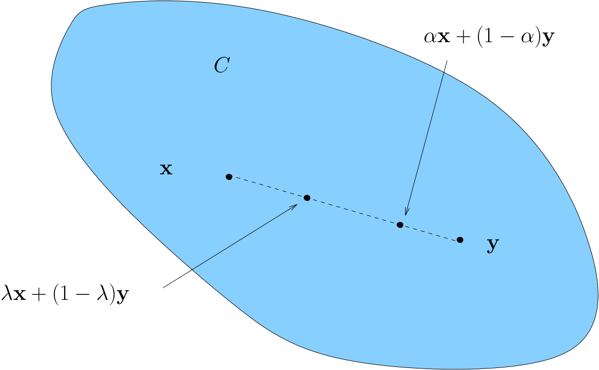
Fig. 74 Convex set

A non-convex set

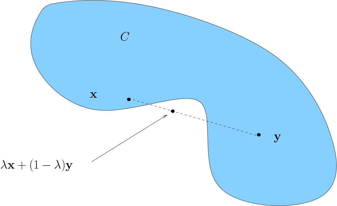
Fig. 75 Non-convex set

Fact about intersection of convex sets

Fact If A and B are convex, then so is A∩B

Define a convex function

f is called (_) if

f(λx+(1−λ)y) ≤ λf(x)+(1−λ)f(y)

for all x,y∈A and all λ∈[0,1]

f is called strictly convex if

f(λx+(1−λ)y)<λf(x)+(1−λ)f(y)

for all x,y∈A with x≠y and all λ∈(0,1)

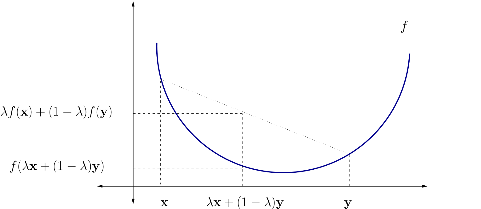
Fig. 76 A strictly convex function on a subset of R#

Fact about convex function

Fact If A is K×K and positive definite, then

Q(x)=x′Ax(x∈R^K)

is strictly convex on R^K

Define a concave function

f is called concave if

f(λx+(1−λ)y) ≥ λf(x)+(1−λ)f(y)

for all x,y∈A and all λ∈[0,1]

f is called strictly concave if

f(λx+(1−λ)y) > λf(x)+(1−λ)f(y)

for all x,y∈A with x≠y and all λ∈(0,1)

Fact

f:A→R is concave if and only if its hypograph (aka subgraph)

H_f:={(x,y)∈A×R:f(x)≥y}

is a convex subset of R^K×R

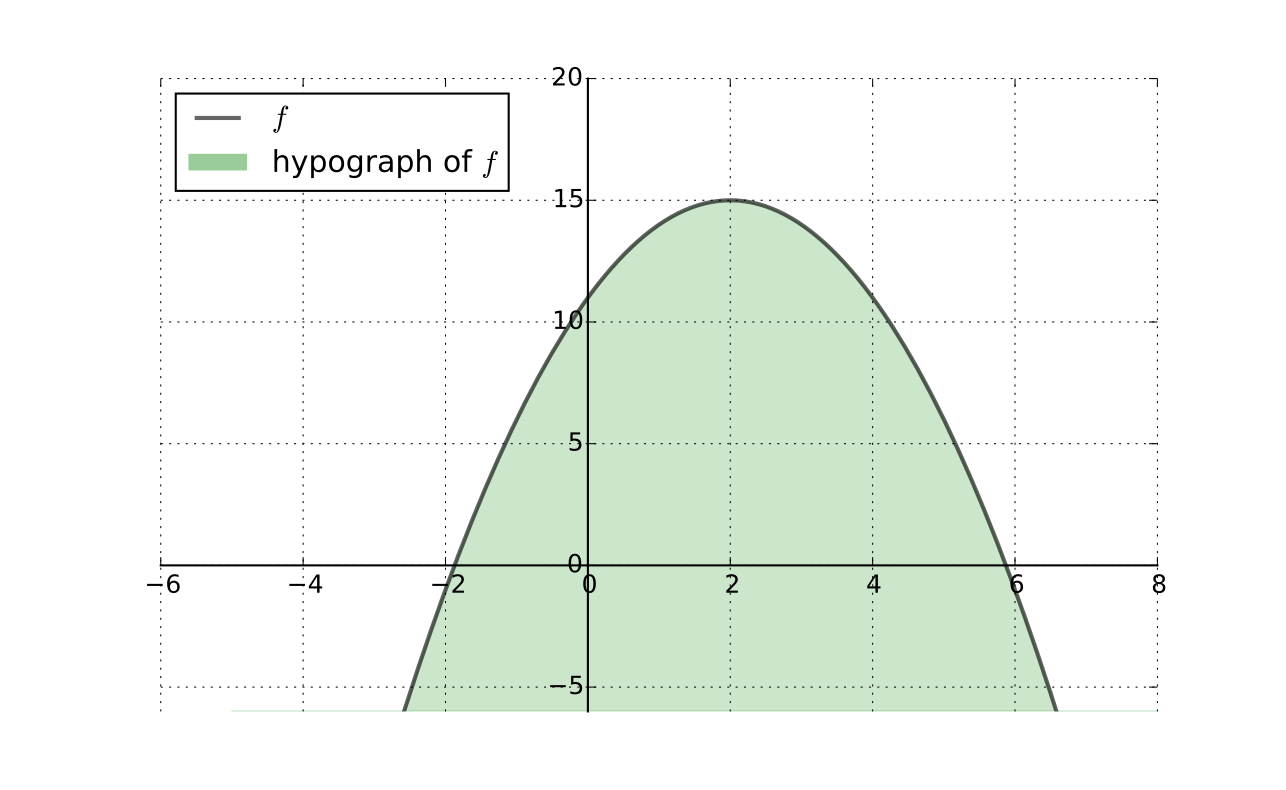
Fig. 79 Convex hypograph/subgraph of a function#

Preservation of Shape

Fact If f and g are convex (resp., concave) and α≥0, then

• αf is convex (resp., concave)

• f+g is convex (resp., concave)

If f and g are strictly convex (resp., strictly concave) and α>0, then

• αf is strictly convex (resp., strictly concave)

• f+g is strictly convex (resp., strictly concave)

Hessian based shape criterion

If f: A→R is a C² function where A⊂RK is open and convex, then

1. Hf(x) positive semi-definite (nonnegative definite) for all x∈A ⟺f convex

2. Hf(x) negative semi-definite (nonpositive definite) for all x∈A ⟺f concave

In addition,

1. Hf(x) positive definite for all x∈A ⟹f strictly convex

2. Hf(x) negative definite for all x∈A ⟹f strictly concave

Advantages of convexity/concavity (two)

1. Sufficiency of first order conditions for optimality

2. Uniqueness of optimizers with strict convexity/concavity

Let A⊂R^K be convex set and let f: A→R be concave/convex differentiable function.

Then x*∈A is a minimizer/minimizer of f on A if and only if x* is a stationary point of f on A.

Uniqueness

Let A⊂R^K be convex set and let f: A→R

1. If f is strictly convex, then f has at most one minimizer on A

2. If f is strictly concave, then f has at most one maximizer on A

Interpretation, strictly concave case:

• we don’t know in general if f has a maximizer

• but if it does, then it has exactly one

• in other words, we have uniqueness

Sufficient and necessary conditions (sets)

Let A⊂R^K be convex set, let f: A→R, and x*∈A stationary, then

1. f strictly concave ⟹ x∗ is the unique maximizer of f on A

2. f strictly convex ⟹ x∗ is the unique minimizer of f on A

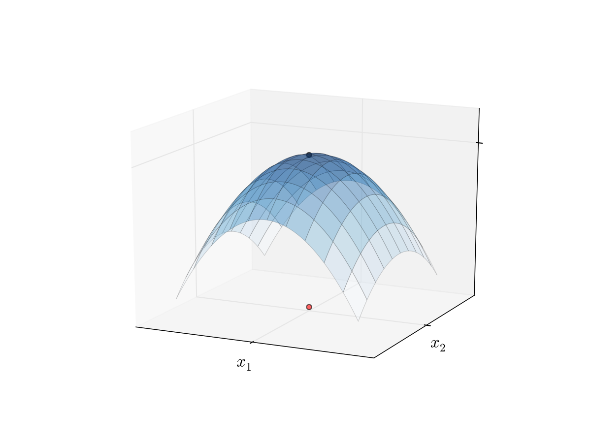
Fig. 80 Unique maximizer for a strictly concave function

Roadmap for unconstrained optimization

1. Assuming that the domain of the objective function is the whole space, check that it is continuous and for derivative based methods twice continuously differentiable

2. Derive the gradient and Hessian of the objective function. If it can be shown that the function is globally concave or convex, checking SOC (below) is not necessary, and global optima can be established

3. Find all stationary points by solving FOC

4. Check SOC to determine whether found stationary points are (local) maxima or minima and filter out saddle points

5. Assess whether any of the local optima are global by comparing function values at these points, and inspecting the shape of the function to determine if its value anywhere exceeds the best local optimum (limits at the positive and negative infinities, possible vertical asymptotes, etc.)

Define the general form of the optimization problem

The (_) is

V(θ)=max_(x) f(x,θ) subject to
g_i(x,θ) = 0, i∈{1,…,I}
h_j(x,θ) ≤ 0, j∈{1,…,J}

where:

• f(x,θ): R^N×R^K → R is an objective function

• x∈R^N are decision/choice variables

• θ∈R^K are parameters

• g_i(x,θ) = 0,i∈{1,…,I} where g_i:R^N×R^K→ R, are equality constraints

• h_j(x,θ) ≤ 0,j∈{1,…,J} where h_j:R^N×R^K→R, are inequality constraints

• V(θ): R^K → R is a value function

State the Lagrange theorem

Let f: R^N → R and g: R^N → R^K be continuously differentiable functions.

Let D={x: g_i(x)=0, i=1,…,K}⊂R^N

Suppose that

• x*∈D is a local extremum of f on D, and

• the gradients of the constraint functions g_i are linearly independent at x* (equivalently, the rank of the Jacobian matrix Dg(x*) is equal to K)

Then there exists a vector λ* ∈ R^K such that

Df(x*)−λ*⋅Dg(x*)=Df(x*)−∑^K_i=1 λ_i*Dg_i(x*)=0

Note on Lagrange

• λ* is called the vector of Lagrange multipliers

• The assumption that the gradients of the constraint functions g_i are linearly independent at x* is called the constraint qualification assumption

• Lagrange theorem provides necessary first order conditions for both maximum and minimum problems

Define the Lagrangian function

Definition

The function L: R^N+K→R defined as

L(x,λ)=f(x)−λ⋅g(x)=f(x)−∑^K_i=1 λ_ig_i(x)

is called a Lagrangian (function)

Hessian of the Lagrangian

Using the rules of the differentiation from multivariate calculus we can express the gradient and the Hessian of the Lagrangian w.r.t. x as

∇_xL(λ,x)=Df(x)−λ⋅Dg(x)H_xL(λ,x)=Hf(x)−λ⊙Hg(x)

• where ⊙ denotes multiplication of the vector λ and the Hessian (K,N,N) tensor Hg(x) along the first dimension

Fact (necessary SOC)

Let f:R^N → R and g: R^N→R^K be twice continuously differentiable functions (C²) and let D = {x: g_i(x)=0,i=1,…,K} ⊂ R^N

Suppose x* ∈ D is the local constrained optimizer of f on D and that the constraint qualification assumption holds at x* and some λ* ∈ R^K

Then:

• If f has a local maximum on D at x*, then H_xL(λ,x) defined above is negative semi-definite on a linear constraint set {v: Dg(x*)v=0}, that is

∀v ∈ R^N and Dg(x*)v=0 ⟹ v′H_xL(λ,x)v≤0

• If f has a local minimum on D at x*, then H_xL(λ,x) defined above is positive semi-definite on a linear constraint set {v: Dg(x*)v=0}, that is

∀v ∈ R^N and Dg(x*)v=0 ⟹ v′H_xL(λ,x)v ≥ 0

Fact (sufficient SOC)

Let f: R^N → R and g: R^N → R^K be twice continuously differentiable functions (C²) and let D={x: g_i(x)=0,i=1,…,K} ⊂ R^N

Suppose there exists x* ∈ D such that rank(Dg(x⋆))=K and Df(x*)−λ*⋅Dg(x*) = 0 for some λ* ∈ R^K (the constraint qualification assumption holds at x* which satisfies the FOC)

Then:

• If H_xL(λ,x) defined above is negative definite on a linear constraint set {v: Dg(x*)v=0}, that is

∀v ≠ 0 and Dg(x*)v = 0 ⟹ v′H_xL(λ,x)v < 0,

then x* is the local constrained maximum of f on D

• If H_xL(λ,x) defined above is positive definite on a linear constraint set {v: Dg(x*)v=0}, that is

∀v ≠ 0 and Dg(x*)v=0⟹v′H_xL(λ,x)v > 0

then x* is the local constrained minimum of f on D

Define bordered Hessian

Definition

The Hessian of the Lagrangian with respect to (λ,x) is called a (_), and is given by

HL(λ,x) = ([0]_K×K [−Dg(x)]_K×N
[−Dg(x)]’_N×K [Hf(x)−λ⊙Hg(x)]_N×N)

Define
a) positive definite subject to a linear constraint
b) negative definite subject to a linear constraint

Definition

Let x ∈ R^N, A is (N×N) symmetric matrix and B is (K×N) matrix.

Quadratic form Q(x) is called positive definite subject to a linear constraint Bx=0 if

Q(x)=x^TAx>0 for all x≠0 and Bx=0

Quadratic form Q(x) is called negative definite subject to a linear constraint Bx=0 if

Q(x)=x^TAx<0 for all x≠0 and Bx=0

Positive and negative semi-definiteness subject to a linear constraint is obtained by replacing strict inequalities with non-strict ones.

recall that Bx=0 is equivalent to saying that x is in the null space (kernel) of B

Definiteness of quadratic form subject to linear constraint table

In order to establish definiteness of the quadratic form x^TAx, x∈R^N, subject to a linear constraint Bx=0, we need to check signs of the N−K leading principle minors of the (N−K×N−K) matrix E which represents the equivalent lower dimension quadratic form without the constraint. The signs of these leading principle minors correspond to (−1)^K times the signs of the determinant of the corresponding bordered matrix H, where a number of last rows and columns are dropped, according to the following table:

Order j of leading principle minor in E	Include first rows/columns of H	Drop last rows/columns of H
1	2K+1	N−K−1
2	2K+2	N−K−2
⋮	⋮	⋮
N−K−1	N+K−1	1
N−K	N+K	0

Clearly, this table has N−K rows, and it is N−K determinants that have to be computed.

The definiteness of the quadratic form subject to the linear constraint is then given by the pattern of signs of these determinants according to the Silvester’s criterion.

Note that computing determinants of H after dropping a number of last rows and columns is effectively computing last leading principle minors of H.

If any of the leading principle minors turns out to be zero, we can move on and check the patters for the semi-definiteness.

Semi-definiteness of quadratic form subject to linear constraint

In order to establish semi-definiteness of the quadratic form x^TAx, x ∈ R^N, subject to a linear constraint Bx=0, we need to check signs of the principle minors of the (N−K×N−K) matrix E which represents the equivalent lower dimension quadratic form without the constraint. The signs of these principle minors correspond to (−1)^K times the signs of the determinant of the corresponding bordered matrix H, where a number number of rows and columns are dropped from among the last N−K rows and columns (in all combinations), according to the following table:

Order j of principle minor in E	Number of principle minors	Drop among last N − K rows/columns
1	N−K	N−K−1
2	C(N−K,2)	N−K−2
⋮	⋮	⋮
N−K−1	N−K	1
N−K	1	0

The table again has N−K rows, but each row corresponds to a different number of principle minors of a given order, namely for order j there are (N−k)-choose-j principle minors given by the corresponding number of combinations C(N−K, j).

The total number of principle minors to be checked is 2N−K−1, given by the sum of binomial coefficients

The definiteness of the quadratic form subject to the linear constraint is then given by the pattern of signs of these determinants according to the Silvester’s criterion.

In what follows we will refer to computing determinants of H after dropping a number of rows and columns among the last N−K rows and columns as computing last principle minors of H. The number of last principle minors will correspond to the number of lines in the table above, and not the number of determinants to be computed.

Fact (definiteness of Hessian on linear constraint set)

Fact

For f: R^N → R and g: R^N → R^K twice continuously differentiable functions (C²):

H_xL(λ,x) is positive definite on a linear constraint set {v: Dg(x*)v = 0} ⟺ the last N−K leading principal minors of HL(λ,x) are non-zero and have the same sign as (−1)^K.

H_xL(λ,x) is negative definite on a linear constraint set {v: Dg(x*)v=0} ⟺ the last N−K leading principal minors of HL(λ,x) are non-zero and alternate in sign, with the sign of the full Hessian matrix equal to (−1)^N.

H_xL(λ,x) is positive semi-definite on a linear constraint set {v:Dg(x*)v=0} ⟺ the last N−K principal minors of HL(λ,x) are zero or have the same sign as (−1)^K.

H_xL(λ,x) is negative semi-definite on a linear constraint set {v:Dg(x*)v=0} ⟺ the last N−K principal minors of HL(λ,x) are zero or alternate in sign, with the sign of the full Hessian matrix equal to (−1)^N.

• see above the exact definition of the last principle minors and how to count them

Fact (necessary SOC)

Let f: R^N → R and g: R^N→R^K be twice continuously differentiable functions (C²), and let D={x: g_i(x)=0,i=1,…,K} ⊂ R^N

Suppose x* ∈ D is the local constrained optimizer of f on D and that the constraint qualification assumption holds at x* and some λ* ∈ R^K

Then:

• If f has a local maximum on D at x*, then the last N−K principal minors of bordered Hessian HL(λ,x) are zero or alternate in sign, with the sign of the determinant of the full Hessian matrix equal to (−1)^N

• If f has a local minimum on D at x*, then the last N−K principal minors of bordered Hessian HL(λ,x) are zero or have the same sign as (−1)^K

• see above the exact definition of the last principle minors and how to count them

Define sufficient SOC for function

Let f: R^N → R and g: R^N → R^K be twice continuously differentiable functions (C²) and let D = {x:g_i(x)=0,i=1,…,K} ⊂ R^N

Suppose there exists x* ∈ D such that rank(Dg(x*))=K and Df(x*)−λ*⋅Dg(x*)=0 for some λ* ∈ R^K (i.e. the constraint qualification assumption holds at (x*,λ*) which satisfies the FOC)

Then:

• If the last N−K leading principal minors of the bordered Hessian HL(λ,x) are non-zero and alternate in sign, with the sign of the determinant of the full Hessian matrix equal to (−1)^N, then x* is the local constrained maximum of f on D

• If the last N−K leading principal minors of the bordered Hessian HL(λ,x) are non-zero and have the same sign as (−1)^K, then x* is the local constrained minimum of f on D

Lagrangian method: algorithm

1. Write down the Lagrangian function L(x,λ)

2. Find all stationary points of L(x,λ) with respect to x and λ, i.e. solve the system of first order equations

3. Derive the bordered Hessian HL(x,λ) and compute its value at the stationary points

4. Using second order conditions, check if the stationary points are local optima

5. To find the global optima, compare the function values at all identified local optima

• note that using convexity/concavity of the objective function is not as straightforward as in the unconstrained case, requires additional assumptions on the convexity of the constrained set

Lagrange method may not work when:

• Constraints qualification assumption is not satisfied at the stationary point

• FOC system of equations does not have solutions (thus no local optima)

• Saddle points – second order conditions can help

• Local optimizer is not a global one – no way to check without studying analytic properties of each problem

Conclusion: great tool, but blind application may lead to wrong results!

Karush-Kuhn-Tucker conditions (maximization)

Let f:RN→R and g:RN→RK be continuously differentiable functions.

Let D={x: g_i(x)≤0, i=1,…,K} ⊂ R^N

Suppose that x⋆∈D is a local maximum of f on D and that the gradients of the constraint functions gi corresponding to the binding constraints are linearly independent at x⋆ (equivalently, the rank of the matrix composed of the gradients of the binding constraints is equal to the number of binding constraints).

Then there exists a vector λ⋆∈RK such that

Df(x⋆)−λ⋆⋅Dg(x⋆)=Df(x⋆)−∑^K_i=1λ*_iDg_i(x*)=0

and

λ_i⋆≥0 with λ_i⋆g_i(x*)=0 i=1,…,K

Karush-Kuhn-Tucker conditions (miminization)

In the settings of KKT conditions (maximization), suppose that x⋆∈D is a local minimum of f on D, and as before the matrix composed of the gradients of the binding constraints has full rank.

Then there exists a vector λ*∈R^K such that (note opposite sign)

Df(x*)+λ*⋅Dg(x*)=Df(x*)+∑^K_i=1λ*_iDg_i(x*)=0

and

λ*_i ≥ 0 with λ*_ig_i(x*)=0 i=1,…,K

• Very similar to the Lagrange theorem, but now we have inequalities!

The general form of the optimisation problem

V(θ)=max_(x)f(x,θ) subject to
g_i(x,θ) = 0, i∈{1,…,I}
h_j(x,θ) ≤ 0, j∈{1,…,J}

where:

• f(x,θ):R^N×R^K → R is an objective function

• x ∈ R^N are decision/choice variables

• θ ∈ R^K are parameters

• g_i(x,θ)=0, i ∈ {1,…,I} where
  g_i:R^N×R^K → R, are equality constraints

• h_j(x,θ)≤0, j ∈ {1,…,J} where
  h_j:R^N×R^K → R, are inequality constraints

• V(θ): R^K→R is a value function

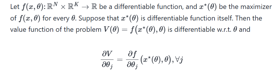
Envelope theorem for unconstrained problems

Let f(x,θ): R^N×R^K→ R be a differentiable function, and x*(θ) be the maximizer of f(x,θ) for every θ. Suppose that x*(θ) is differentiable function itself. Then the value function of the problem V(θ)=f(x*(θ),θ) is differentiable w.r.t. θ and

∂V/∂θ_j= (∂f/∂θ_j) (x*(θ),θ),∀j

Envelope theorem for constrained problems

Consider an equality constrained optimization problem

V(θ)=max_(x)f(x,θ) subject to g_i(x,θ)=0,i∈{1,…,I}

where:

• f(x,θ): R^N×R^K→R is an objective function

• x ∈ R^N are decision/choice variables

• θ ∈ R^K are parameters

• g_i(x,θ)=0, i∈{1,…,I} where g_i: R^N×R^K → R, are equality constraints

• V(θ): R^K → R is a value function

Assume that the maximizer correspondence D*(θ) = argmax f(x,θ) is single-valued and can be represented by the function x*(θ): R^K → R^N, with the corresponding Lagrange multipliers λ*(θ): R^K→R^I.

Assume that both x*(θ) and λ*(θ) are differentiable, and that the constraint qualification assumption holds. Then

∂V/∂θ_j=(∂L/∂θ_j)(x*(θ),λ*(θ),θ), ∀j

where L(x,λ,θ) is the Lagrangian of the problem.