ST442 - Longitudinal Data Analysis

What is a longitudinal study?

A study that tracks the same group of subjects over time — may be individuals, countries, or organizations

What is the difference between a cohort study and a panel study?

A cohort study follows a group who experience a common event (e.g. same birth year); a panel study follows a cross-section of the population over time.

What are two types of longitudinal data?

1. Repeated measures — same variable measured at multiple times

2. Event history — time until an event occurs (e.g. marriage to divorce)

What are two advantages of longitudinal data over cross-sectional data?

• 1. Can separate within-subject from between-subject variance.

  • i.e. Large variation in political attitudes btwn people, little change in an individual’s attitudes over time).

  • Can focus on within-subj change more precisely after adjusting for btwn-subj differences.

• 2. A subject can act as its own control, e.g. in cross-over experiments or observational studies

  • cross-over: individual switches between treatment and control over time.

  • observational: examine how outcome Y varies with change in X controlling for unmeasured time-invariant subject characteristics.

• 3. Separate different sorts of time effect: period, age, cohort

• 4. Can explore within-subject chaange and amount of variation in change across subjects

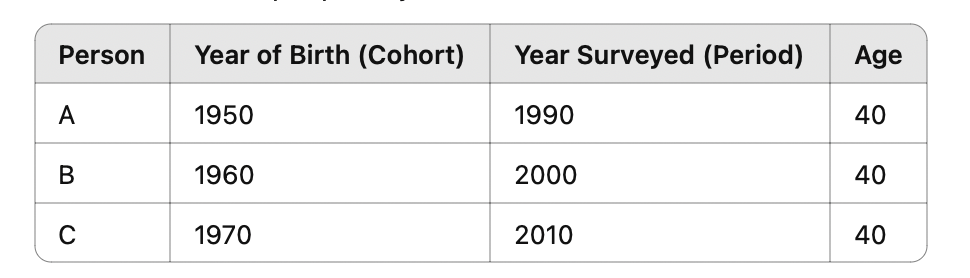
What are the three types of time effects in longitudinal data?

1. Age

2. Period

3. Cohort

Note A = P - C. We cannot identify all 3 effect if all are linear bc linearly independent. This perfect linear dependency makes it impossible to estimate all three effects simultaneously in a regression model without some constraint or assumption — the model would suffer from perfect multicollinearity.

Age effect

How individuals change as they get older

Does a person’s support for capital punishment increase as they get older?

Period effect

How events at specific calendar times affect all individuals  

A high-profile miscarriage of justice case in year t might reduce support for CP.

Cohort effect

 How being born in a particular time period shapes attitudes over time

Were attitudes at age 40 the same for people born in 1940 and in 1970?

What challenges are there with longitudinal data?

1. Follow-up is costly and difficult, so attrition is a major problem

2. More sophisticated analysis required to account for within-subject correlation in Y

3. Risk of feedback effects and unmeasured cofounders in ‘causal’ effects.

Effects of attrition

Follow-up is costly and difficult, and drop-out (attrition) can reduce sample size and cause bias due to selective attrition.

Selective attrition occurs when drop-outs differ systematically from those who remain, potentially biasing estimates if related to unmeasured factors influencing Y.

Why can't causal inference be made using cross-sectional data?

Causal inference is not possible using cross-sectional data unless treatment is randomly allocated.

This is because cross-sectional data only provides a snapshot in time, making it challenging to determine the direction or existence of any causal relationships. Without longitudinal data to track changes over time, we cannot be certain if the observed relationships reflect true causality.

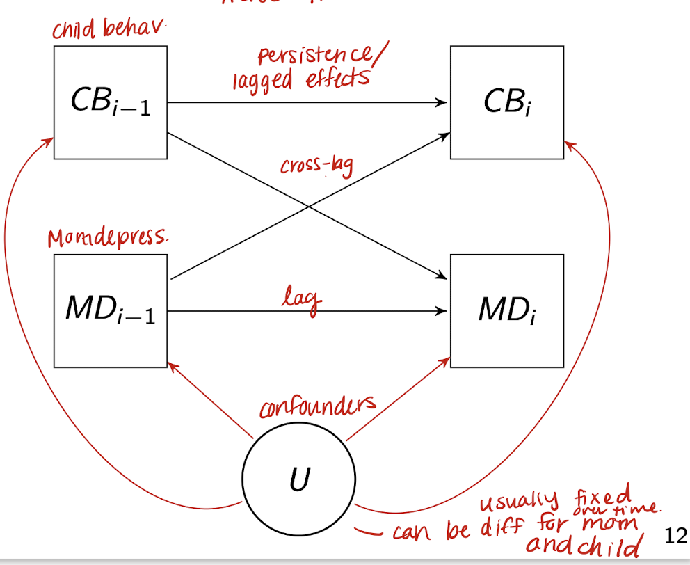
What dynamics are at play in the longitudinal relationship between child behavior (CB) and maternal depression (MD), and how can longitudinal data analysis (LDA) help?

• CB and MD can influence each other over time through reciprocal (cross-lagged) effects.

• CB at time i-1 may affect both CB and MD at time i, and similarly for MD.

• Unmeasured confounders (e.g., genetic or environmental factors) may affect both variables at multiple time points.

• Longitudinal data analysis (LDA) allows researchers to model these temporal relationships and disentangle directionality, lagged effects, and within-subject correlations, helping to clarify—but not prove—causal pathways.

What are anticipatory effects in longitudinal data, and why do they complicate causal inference?

* Anticipatory effects = lag between decisions and behavior

* Mental health may decline before divorce

* Could mean MH → divorce

* But maybe marital problems → MH → divorce

* We usually observe events (e.g. divorce)

* But not the prior changes (e.g. relationship quality)

* Makes it hard to know what really caused what

y_{ij}

* Response for subject j

* At occasion (time point) i

* i = 1, \dots, T_j — number of times subject j is observed

* j = 1, \dots, n — total number of subjects

What does N represent in longitudinal data?

* Total number of observations

* N = \sum_{j=1}^{n} T_j

* Sum of all observations across all subjects and time points

* Represents the overall dataset size available for analysis, which helps in estimating the stability and reliability of statistical conclusions in longitudinal studies.

What does t_{ij} represent in longitudinal data?

* Timing of measurement occasion i for subject j

* Can vary across subjects and occasions

What does x_{ij} represent in longitudinal data?

* Time-varying covariate for subject j at time i

* Can change over time

* Also called predictor, explanatory variable, or independent variable

What does x_j represent in longitudinal data?

* Time-invariant covariate for subject j

* Does not vary over time (i.e. race)

* Subject-specific characteristic

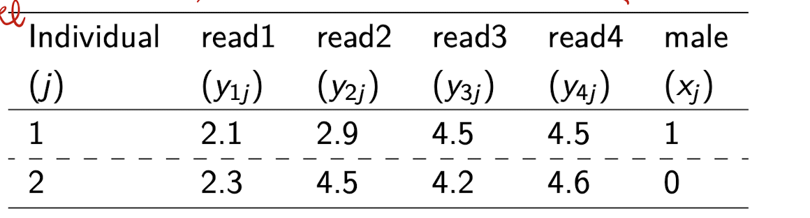
When should data be in wide form?

Structural equation modelling approaches

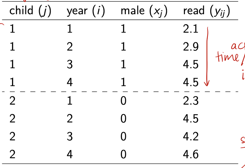
When should data be in long form?

Most method of LDA require long form. This format facilitates the analysis of repeated measurements and accounts for the correlation of observations within subjects.

Why can’t we just use standard regression?

* Assumes \epsilon_{ij} \sim N(0, \sigma^2)

* Assumes independence: \text{Cov}(\epsilon_{ij}, \epsilon_{i'j}) = 0 for i \ne i'

* Treats all nT observations as independent → problematic

* standard errors underestimated → underestimation of p-values, reject null when we should not

Why is the independence of error terms assumption problematic in longitudinal data?

* Repeated observations come from the same subject

* Responses are likely correlated within subjects

* Violates the i.i.d. assumption of OLS

What is the formula for the sample mean standard error under independence?

* \text{SE}(\bar{Y}) = \frac{\text{sd}(Y)}{\sqrt{nT}}

* Assumes all nT observations are independent

* Leads to SE that is too small if this assumption is violated

What happens to standard error if the independence assumption is violated?

* nT overstates the amount of independent info

* Use a smaller “effective sample size” (ESS) instead

* SE should be: \text{SE}(\bar{Y}) = \frac{\text{sd}(Y)}{\sqrt{\text{ESS}}}

What is the effective sample size (ESS)?

* Estimate of the number of truly independent observations

* Reflects loss of information due to clustering or correlation

* Used to correct standard errors

-

* \text{ESS} = nT — assumes no clustering

* \text{ESS} = n — perfect clustering (no within-subject variation)

Why is \text{ESS} = n in the case of perfect clustering?

* All responses from the same subject are identical

* No individual-level variance: y_{ij} = y_j

* Only subject-level info contributes to inference

What are limitations of standard regression models for longitudinal data?

* Can't separate within-subject vs. between-subject variance in y

* Can't explore between-subject differences in change over time

* OLS estimator is biased for dynamic panel models

(e.g. when past values of y are included as predictors)

What are three major methods for analyzing repeated measures in longitudinal data?

* Growth curve models — focus on individual change over time using subject-specific curves

* Marginal models — focus on population-averaged effects, adjusting SEs for within-subject dependence

* Dynamic panel models — include lagged outcomes as predictors to study state dependence and unobserved heterogeneity

What are growth curve models used for in repeated measures analysis?

* Fit a curve to each subject’s repeated measures

* Capture between-subject differences in level and change in y

* Use random effects to account for individual variation

* Can be framed as multilevel or structural equation models

* Variants: latent class growth analysis, growth mixture models

What are marginal models used for in repeated measures analysis?

* Focus on estimating average effects (population-level)

* Allow for within-subject dependence in y

* Treat that dependence as a nuisance (not modeled explicitly)

* Adjust SEs to correct for clustering

* Often used for binary outcomes

What are dynamic panel models used for in repeated measures analysis?

* Also called autoregressive or lagged response models

* Include past y as a predictor of current y

* Distinguish:

- State dependence (effect of past y)

- Unobserved heterogeneity (stable subject traits)

* Subject effects can be fixed or random

* Useful in causal inference, e.g., maternal depression example

What is the special case of T = 2 repeated measures, and when is it used?

* Also called the two-wave or pretest-posttest design

* Subjects observed before and after a treatment or intervention

* Common in experimental or quasi-experimental studies

* Can also apply to naturally occurring events (e.g. divorce, job loss)

What is a pretest-posttest design?

* A type of two-wave design

* Measures outcomes before (pretest) and after (posttest) an intervention

* Helps assess change attributable to the intervention

How are treatment groups defined in two-wave designs?

* Treatment assignment can be random or nonrandom

* May occur in experiments, quasi-experiments, or observational studies

* 'Treatment' can be an event or a continuous variable (e.g. income level)

What is the notation for a two-wave pretest-posttest design?

* x_j = binary treatment indicator (1 = treated, 0 = control)

* y_{1j} = pretest score for subject j

* y_{2j} = posttest score for subject j

* More generally, x_j can be any predictor, not just treatment

What are the two main modeling approaches for T = 2 repeated measures?

* Lagged response model — model posttest y_{2j} controlling for pretest y_{1j}

* Change score model — model the difference: d_j = y_{2j} - y_{1j}

-

* Both estimated via OLS

* Both estimate the treatment effect of x on y

What is the lagged response model for T = 2 data?

* Model: y_{2j} = \alpha + \beta y_{1j} + \delta x_j + e_j

* y_{1j} = pretest score, x_j = treatment, y_{2j} = posttest score

* Controls for pretest score to isolate treatment effect \delta

* Assumes \text{cov}(e_j, x_j) = \text{cov}(e_j, y_{1j}) = 0

* Assumes: e_j \sim N(0, \sigma^2) and uncorrelated with x_j, y_{1j}

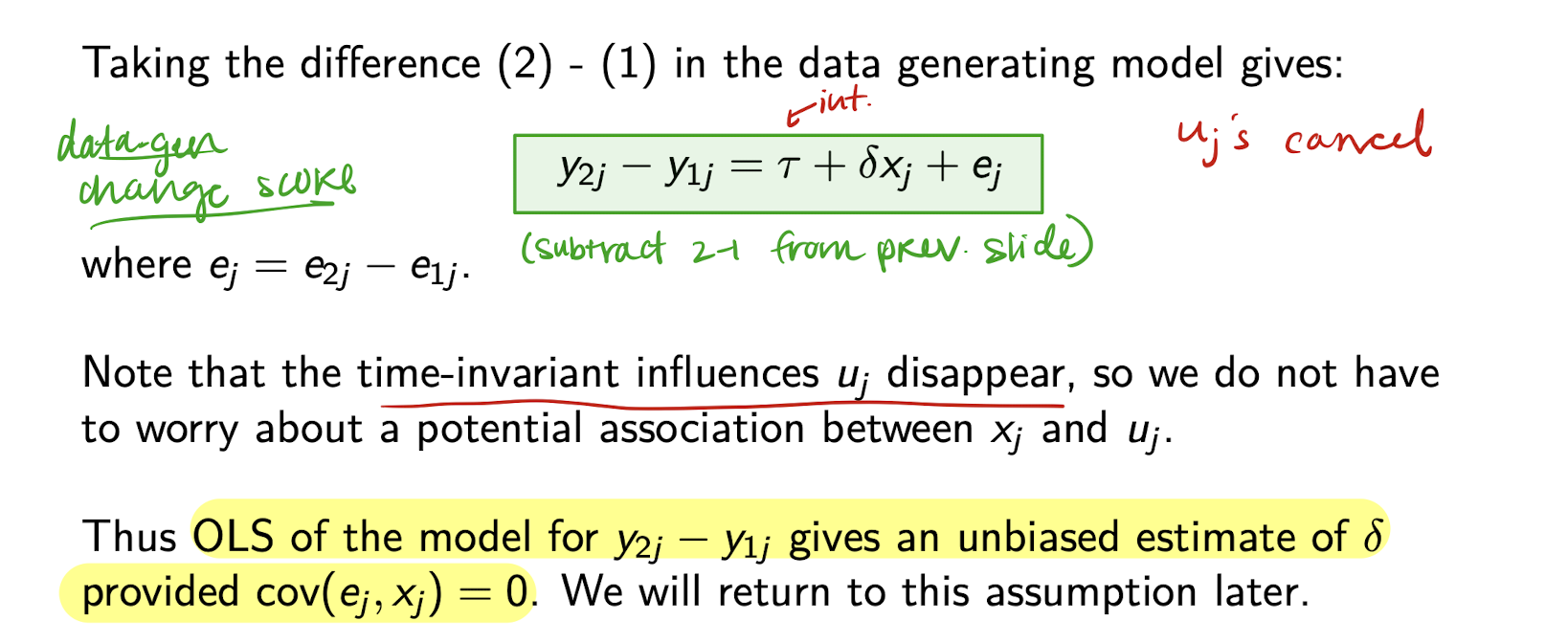
What is the change score model for T = 2 data?

* Model: d_j = y_{2j} - y_{1j} = \tau + \delta x_j + e_j

* Uses the difference between posttest and pretest

* Focuses directly on change in y

* Assumes: \text{cov}(e_j, x_j) = 0

* Assumes: e_j \sim N(0, \sigma^2) and uncorrelated with x_j

* Only one predictor: x_j

Why adjust for pretest if subjects are randomly allocated to treatment?

* On average, groups will have equal pretest means

* But differences may still occur by chance in a given experiment

* Adjusting for pretest accounts for this

* Must be done carefully to avoid bias from regression to the mean

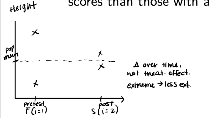
What is regression to the mean (RTM)?

* Extreme values tend to be followed by less extreme ones

* Happens due to random variation (e.g., luck, illness)

* Individuals with high or low y_1 tend to show larger changes in y

How does RTM affect interpretation in the change score model?

* Individuals with extreme y_1 will regress toward the mean

* This can exaggerate or mask treatment effects

* Particularly problematic when pretest means differ across groups

What is the formula for the treatment effect estimate in the change score model?

* \hat{\delta} = (\bar{y}_{2T} - \bar{y}_{2C}) - (\bar{y}_{1T} - \bar{y}_{1C})

* Subtracts pretest difference from posttest difference

* Helps isolate change due to treatment, adjusting for initial imbalance

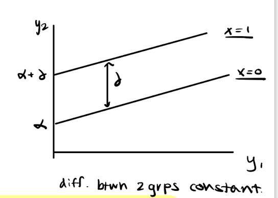
Why is the lagged response model not affected by regression to the mean (RTM)?

* Model: y_{2j} = \alpha + \beta y_{1j} + \delta x_j + e_j

* Fits two parallel lines: one for each group (x = 0, x = 1)

* \delta = expected difference in y_2 for any y_1

* Does not rely on group mean differences in y_1 or y_2

* So estimate of \delta is unaffected by RTM

* The lagged response model accounts for individual differences in response and does not rely on mean group differences, making it resilient to issues caused by regression to the mean.

How should you choose between lagged response and change score models when x is not randomly assigned?

• If x is random and \bar{y}_{1T} \approx \bar{y}_{1C} →

  • Either model is fine (or use posttest difference)

  • LR model helps improve precision

• If x is random but \bar{y}_{1T} \ne \bar{y}_{1C} →

  • CS model is biased due to RTM

  • LR model gives unbiased \delta and adjusts for y_1

• If x is nonrandom →

  • Situation is like an observational study

  • Careful model choice is needed

  • Now enter realm of quasi-experiments or non-equivalent group designs

Example of DGP of graduate salaries

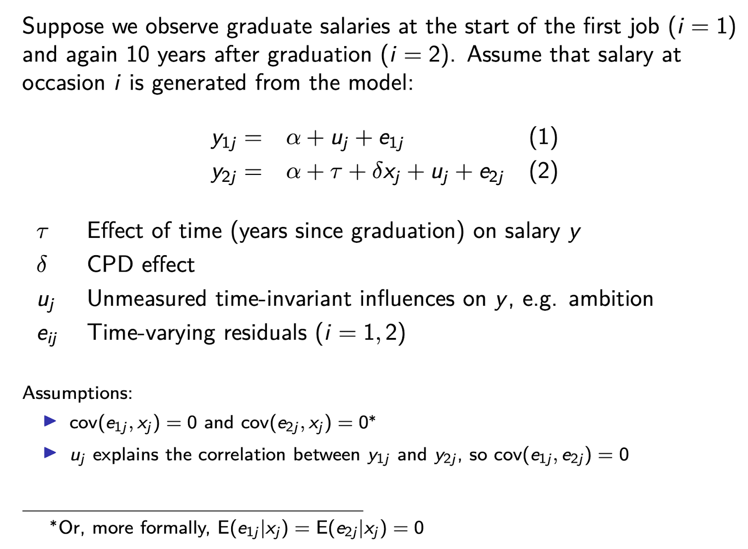
Correlation between u_j and x_j

unmeasured time-invariant characteristics u_j may influence x_j as well as y_{ij}

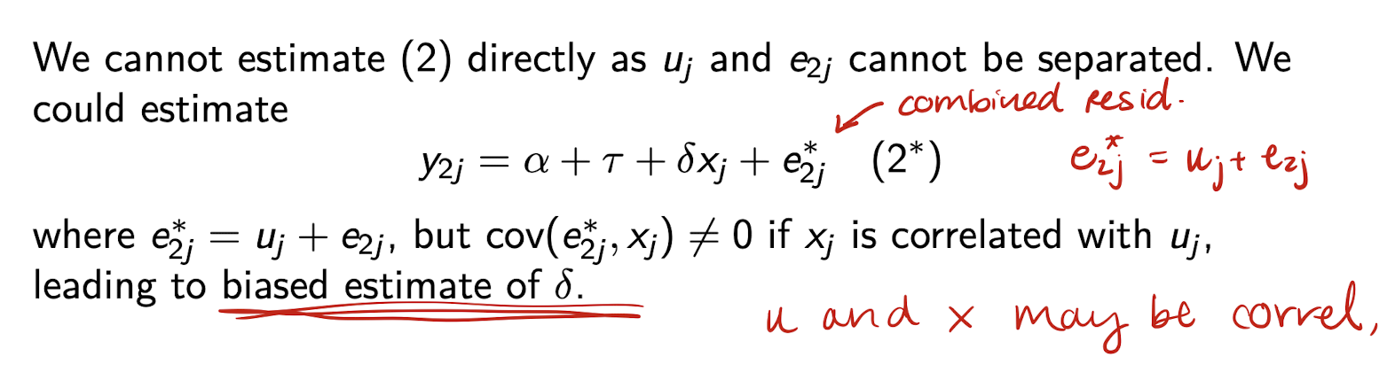
What is an unbiased estimate of the change score model?

What is the implied lagged response model?

* Rearranged form:

y_{2j} = \alpha^* + \beta y_{1j} + \delta x_j + e_j^*

where:

e_j^* = u_j(1 - \beta) + e_{2j} - \beta e_{1j}

* u_j does not cancel out

* Bias in \delta unless:

(i) \text{Cov}(e_j^*, x_j) = 0

(ii) \text{Cov}(e_j^*, y_{1j}) = 0

How does the change score model eliminate u_j?* Subtract:

y_{2j} - y_{1j} = \tau + \delta x_j + e_j

where e_j = e_{2j} - e_{1j}

* u_j cancels out

* Removes time-invariant bias

* Estimate of \delta is unbiased if

\text{Cov}(e_j, x_j) = 0

Which model is better when x_j is non-random?

* Change score model removes u_j

→ Less biased under time-invariant confounding

* Lagged response model keeps u_j

→ Risk of bias if u_j is correlated with x_j or y_{1j}

* Use CS model if

\text{Cov}(e_j, x_j) = 0

is more plausible than

\text{Cov}(e_j^*, x_j) = 0 and

\text{Cov}(e_j^*, y_{1j}) = 0

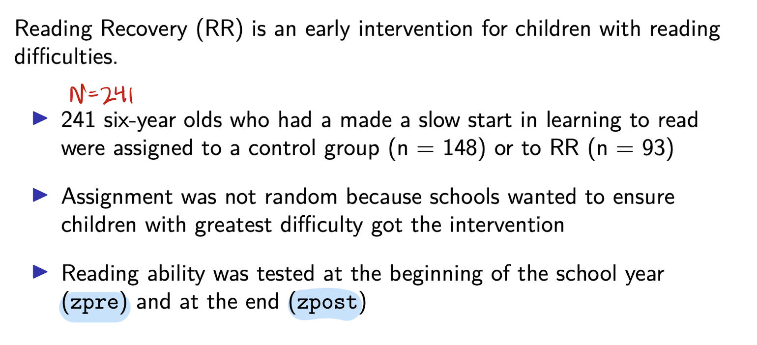
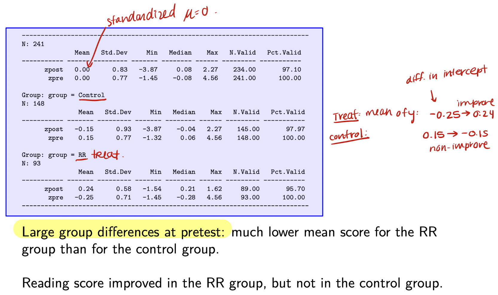
Pretest-posttest example: Reading Recovery

Reading Recovery: regression output from CS model

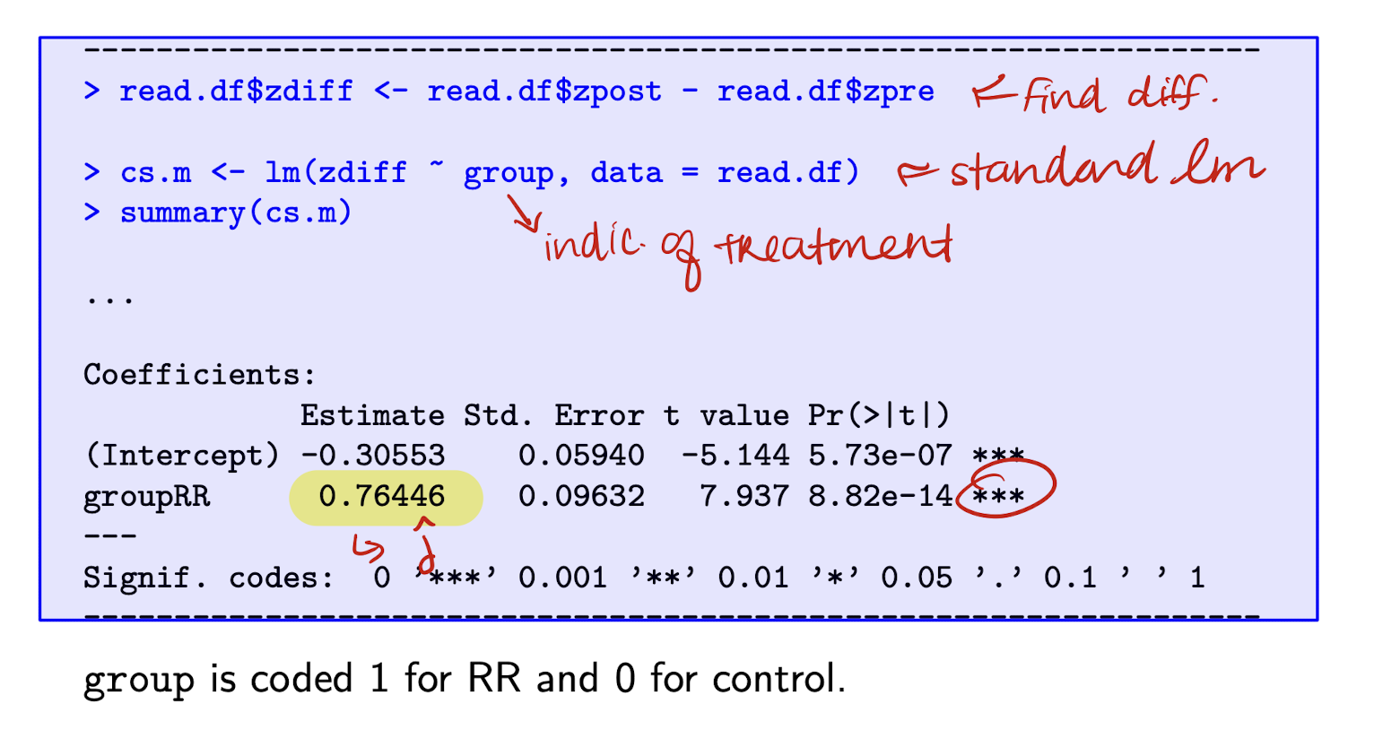
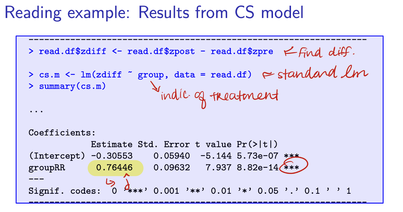
Interpret \hat{\delta}

The posttest-pretest difference is expected to be 0.76 points higher for the RR group than the control group.

Reading Recovery: regression output from LR model

Note that zpre is now a control. A potential u_j may be cognitive ability (time-invariant confounder) and it is correlated with treatment, becuase ability determines whether you’re selected into RR group → bias in LR model. PRE-TEST (X) NON-RANDOMLY ALLOCATED.

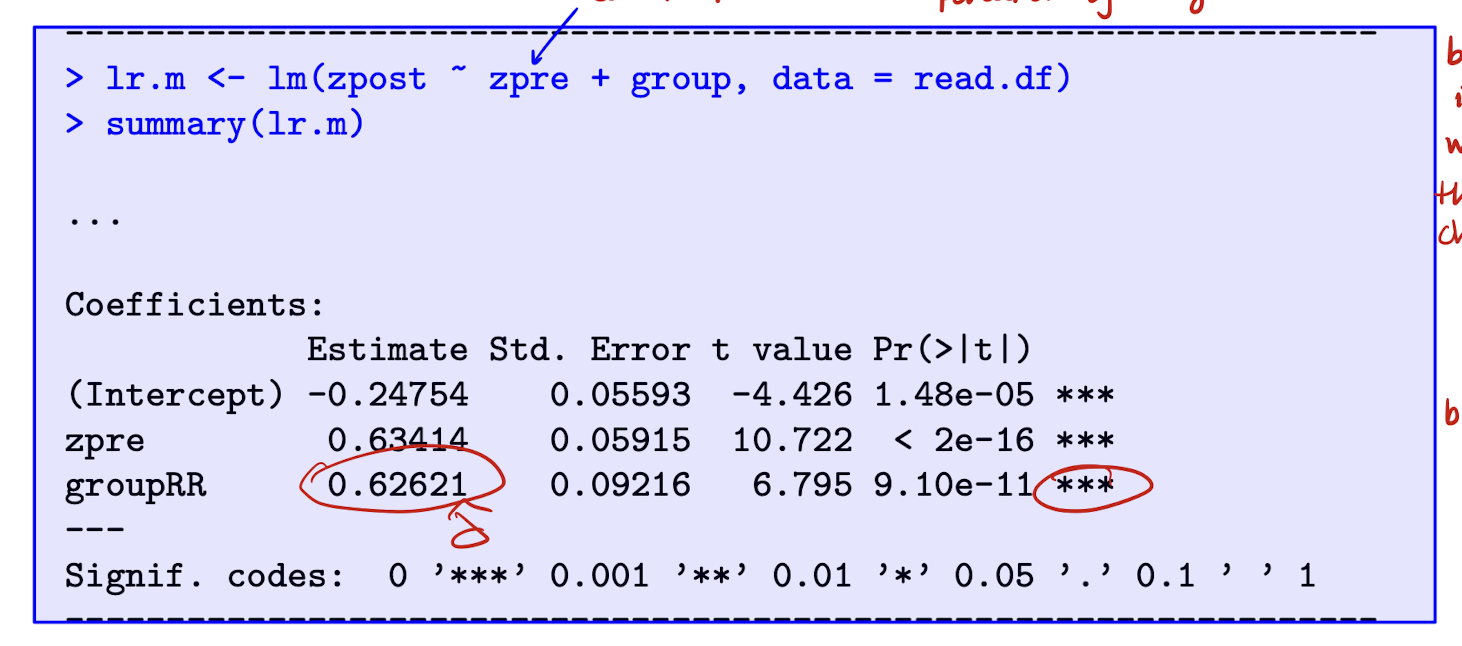
Interpret \hat{\delta}

Conditional on their pretest reading score, children in RR group are expected to score 0.63 points higher in the posttest than those in control group.

When is it appropriate to use the Lagged Response (LR) model for non-random x?

* Use LR model cautiously, but it may help when:

(i) Treatment assignment depends on y_{1j},

especially its time-varying part e_{1j} (not u_j)

(ii) Treatment effect may vary by pretest score y_{1j}

→ Suggests interaction between x and y_{1j}

(iii) You believe y_{1j} causally affects y_{2j}

→ Important to model y_{1j} directly

Why can the change score model be biased when treatment depends on e_{1j}?

* CS model:

y_{2j} - y_{1j} = \tau + \delta x_j + (e_{2j} - e_{1j})

* OLS is unbiased if:

\text{Cov}(e_{ij}, x_j) = 0 for i = 1, 2

* But if x_j depends on y_{1j} or its time-varying part e_{1j}

→ Then \text{Cov}(e_{1j}, x_j) \ne 0

→ Biases estimate of \delta

* CS model ignores time-invariant confounding,

but is still vulnerable to time-varying confounders

When should you use the LR model if the treatment effect depends on y_{1j}?

* Both CS and LR models assume a constant treatment effect

* But if the effect of x_j depends on y_{1j}, you need an interaction

* In LR model:

y_{2j} = \alpha + \beta_0 y_{1j} + \delta_0 x_j + \delta_1 x_j y_{1j} + e_j

→ Treatment effect = \delta_0 + \delta_1 y_{1j}

* Can't model this interaction in CS model (no y_{1j} on RHS)

* Use LR model when you expect the treatment effect to vary with pretest scores

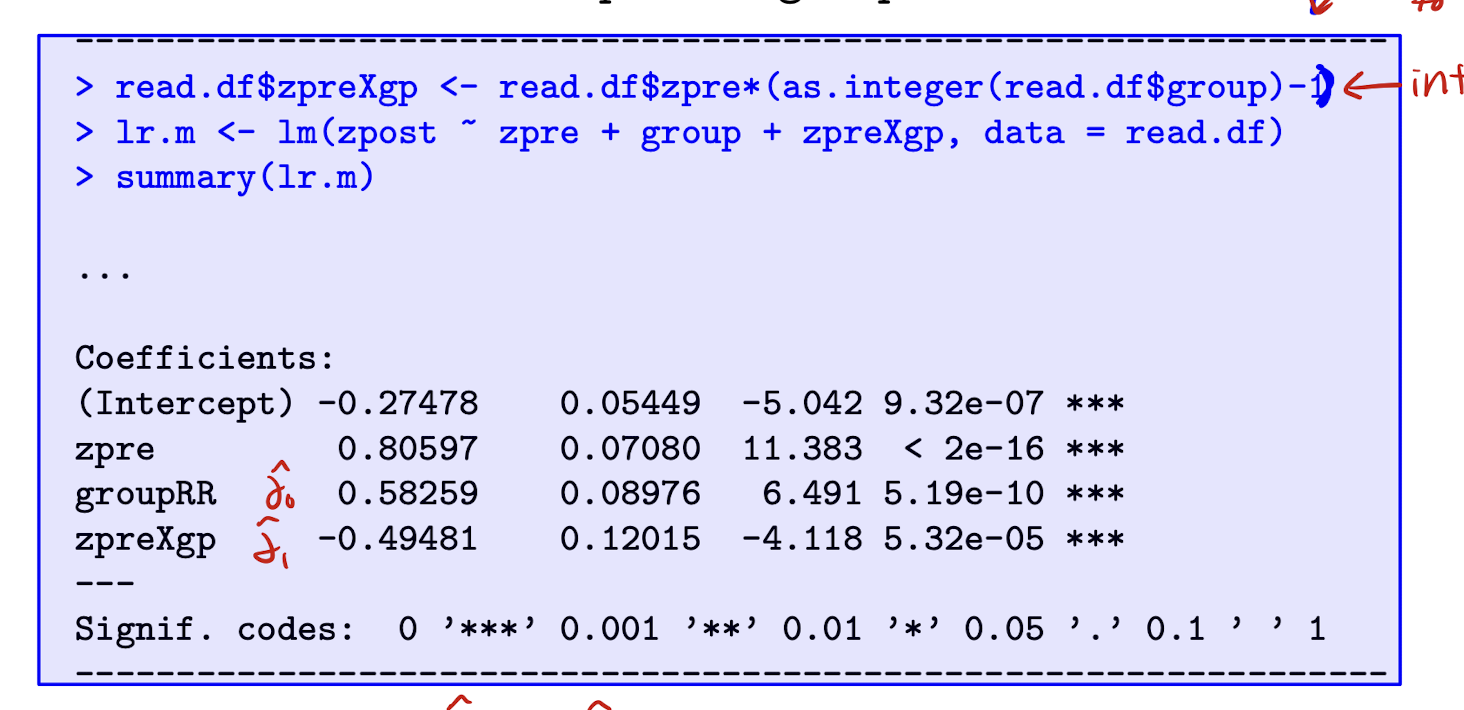
Reading Recovery: LR model w/ interaction. Interpret \hat{\delta}

The effect of RR is estimated as \hat{\delta_0} + \hat{\delta_1} y_{1j} = 0.583 - 0.495 * zpre, so smaller effect for children who had higher test scores at pre-test.

When should you use the LR model if y_1 causally affects y_2?

* If y_1 directly influences y_2

(e.g., salary, weight, enrollment), LR matches the data-generating process

* Examples:

- Salary at time 1 affects salary at time 2 via raises

- Body weight at one time affects weight later

- Prior enrollment affects future course registration

* LR model explicitly includes y_1 as a predictor

→ Captures state dependence

* Helps distinguish:

- Direct effect of y_1 on y_2

- vs. effect of unmeasured traits like ambition or health

Summary: When is the lagged response (LR) model appropriate for non-random x_j?

1. Treatment x_j depends on e_{1j}

- x_j = treatment indicator for subject j

- e_{1j} = time-varying error at pretest (e.g. random shock to y_1)

- If \text{Cov}(e_{1j}, x_j) \ne 0 → CS model is biased

2. Treatment effect varies by pretest score y_{1j}

- y_{1j} = pretest outcome (e.g. salary at time 1)

- Include interaction x_j \cdot y_{1j} in LR model to allow effect to vary

3. Pretest score y_{1j} causally affects posttest y_{2j}

- y_{2j} = posttest outcome (e.g. salary at time 2)

- LR model includes y_{1j} on RHS → captures state dependence

How is the repeated measures ANOVA (fixed effects) model related to the CS model?

* Model:

y_{ij} = \alpha + \tau_i + \delta x_{ij} + u_j + e_{ij}

- y_{ij} = outcome for subject j at time i

- x_{ij} = treatment indicator (e.g. 0 at time 1, x_j at time 2)

- \tau_i = time effect (categorical, e.g. \tau_1 = 0)

- u_j = subject effect (fixed, like a dummy)

- e_{ij} = error term

* u_j treated as a fixed coefficient

→ like including a dummy for each subject

* Equivalent to CS model with:

y_{1j} = \alpha + u_j + e_{1j}

y_{2j} = \alpha + \tau + \delta x_j + u_j + e_{2j}

→ Combine to form:

y_{ij} = \alpha + \tau_i + \delta x_{ij} + u_j + e_{ij}

* Fixed effects ANOVA is just the CS model in long form with subject and time dummies.

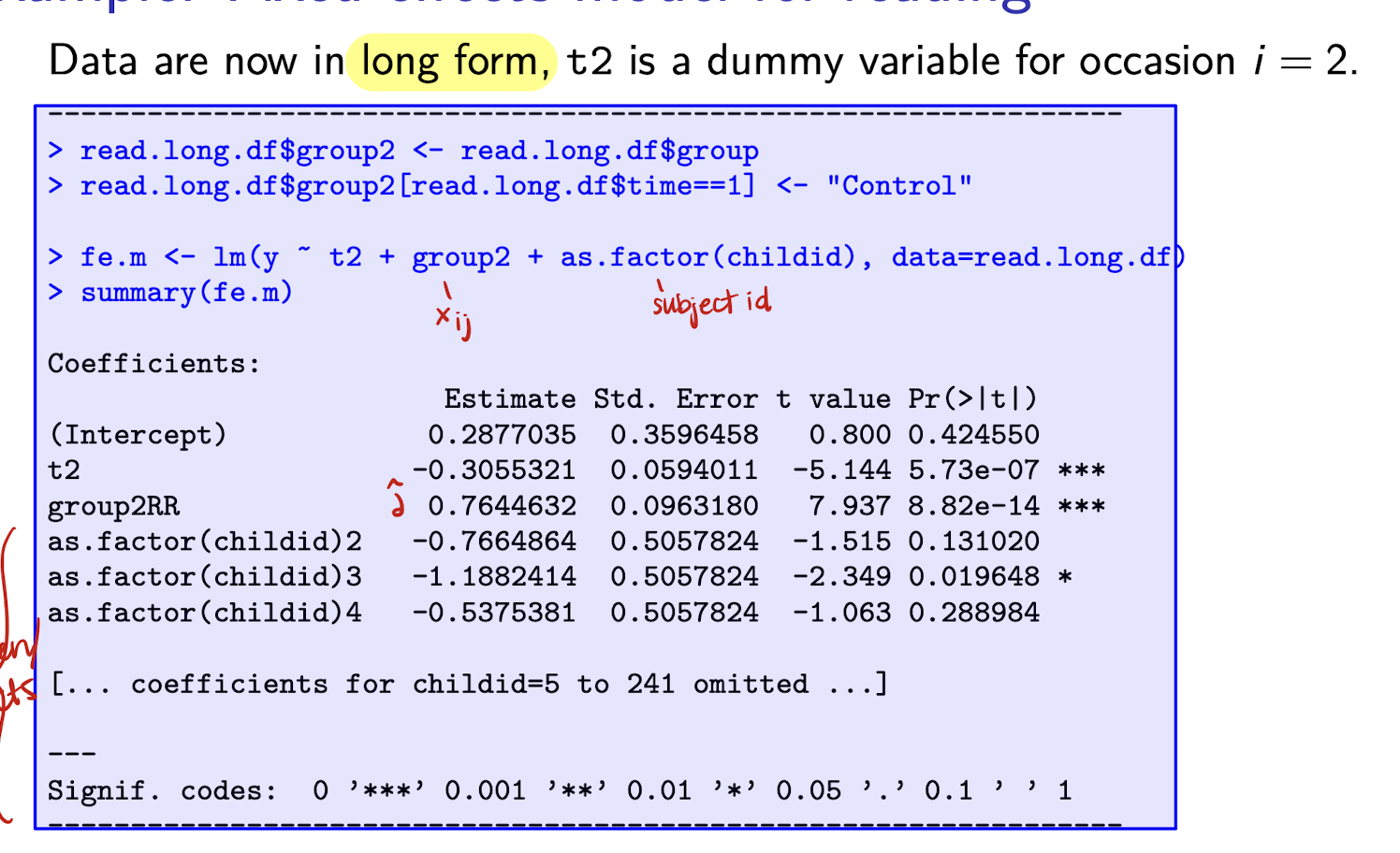
Reading Recovery: Fixed effects model (CS model)

The estimated coefficient of group2RR and its SE are identical to that of groupRR from the CS model.

How do we express the fixed effects model using subject dummies?

* Model:

y_{ij} = \alpha + \tau_i + \delta x_{ij} + \sum_{k=2}^n u_k d_{ik} + e_i

- y_{ij} = outcome for subject j at time i

- \tau_i = time effect (e.g. \tau_1 = 0)

- x_{ij} = treatment (e.g. x_j at time 2)

- u_k = subject fixed effect for subject k

- d_{ik} = 1 if i = k, 0 otherwise

- e_i = error term

* \sum u_k d_{ik} = set of individual dummy variables

- This is a long way of writing the fixed effects for each subject

* First subject is reference (no dummy for k=1)

What is the repeated measures model with random subject effects (Random Effects model)

* Model:  

  y_{ij} = \alpha + \tau_i + \delta x_{ij} + u_j + e_{ij}  

  - y_{ij} = outcome for subject j at time i  

  - \tau_i = time effect (categorical/time dummy)  

  - x_{ij} = treatment or predictor variable  

  - u_j \sim N(0, \sigma_u^2) = random subject effect  

  - e_{ij} \sim N(0, \sigma_e^2) = residual error

This is called a random effects model because u_j is random.

What assumptions for Random Effects model?

  - \text{Cov}(u_j, x_{ij}) = 0  

  - \text{Cov}(e_{ij}, x_{ij}) = 0

• Random effects are uncorrelated with the predictors used in the model.

In other words, the individual random effects must not be related to the treatment or predictor variables to ensure unbiased estimation.

What is intra-class correlation in the random effects model?

* Intra-class correlation (ICC), also called the variance partition coefficient:

\rho = \frac{\sigma_u^2}{\sigma_u^2 + \sigma_e^2}

In other words, it’s is variance between subjects/total variance.

Answers the q: how much remaining variance is due to unexplained variance between individuals?

* \rho measures:

- Correlation between two observations from the same subject

- Proportion of total variance explained by subject-level effects

- How much of the remaining variance is due to between-subject variation

How do we derive the intra-class correlation coefficient \rho?

* \rho measures the correlation between two responses y_{1j} and y_{2j} from the same person, conditional on x.

* Start with the correlation formula:

\rho = \frac{\text{Cov}(u_j + e_{1j},\ u_j + e_{2j})}{\sqrt{\text{Var}(u_j + e_{1j}) \cdot \text{Var}(u_j + e_{2j})}}

-

* Expand the numerator using linearity of covariance:

\text{Cov}(u_j + e_{1j},\ u_j + e_{2j}) = \text{Cov}(u_j, u_j) + \text{Cov}(u_j, e_{2j}) + \text{Cov}(e_{1j}, u_j) + \text{Cov}(e_{1j}, e_{2j})

-

* Under the assumptions:

* \text{Cov}(u_j, e_{ij}) = 0 (for all i),

* \text{Cov}(e_{1j}, e_{2j}) = 0 (independence of errors),

the only non-zero term is \text{Cov}(u_j, u_j) = \text{Var}(u_j) = \sigma_u^2

-

* Now compute the denominator:

\text{Var}(u_j + e_{ij}) = \text{Var}(u_j) + \text{Var}(e_{ij}) = \sigma_u^2 + \sigma_e^2

* So both terms in the denominator are \sigma_u^2 + \sigma_e^2, and the square root of their product is \sigma_u^2 + \sigma_e^2

-

* Final result:

\rho = \frac{\sigma_u^2}{\sigma_u^2 + \sigma_e^2}

* Interpretation: Proportion of residual variance explained by between-individual differences (i.e. subject effects).

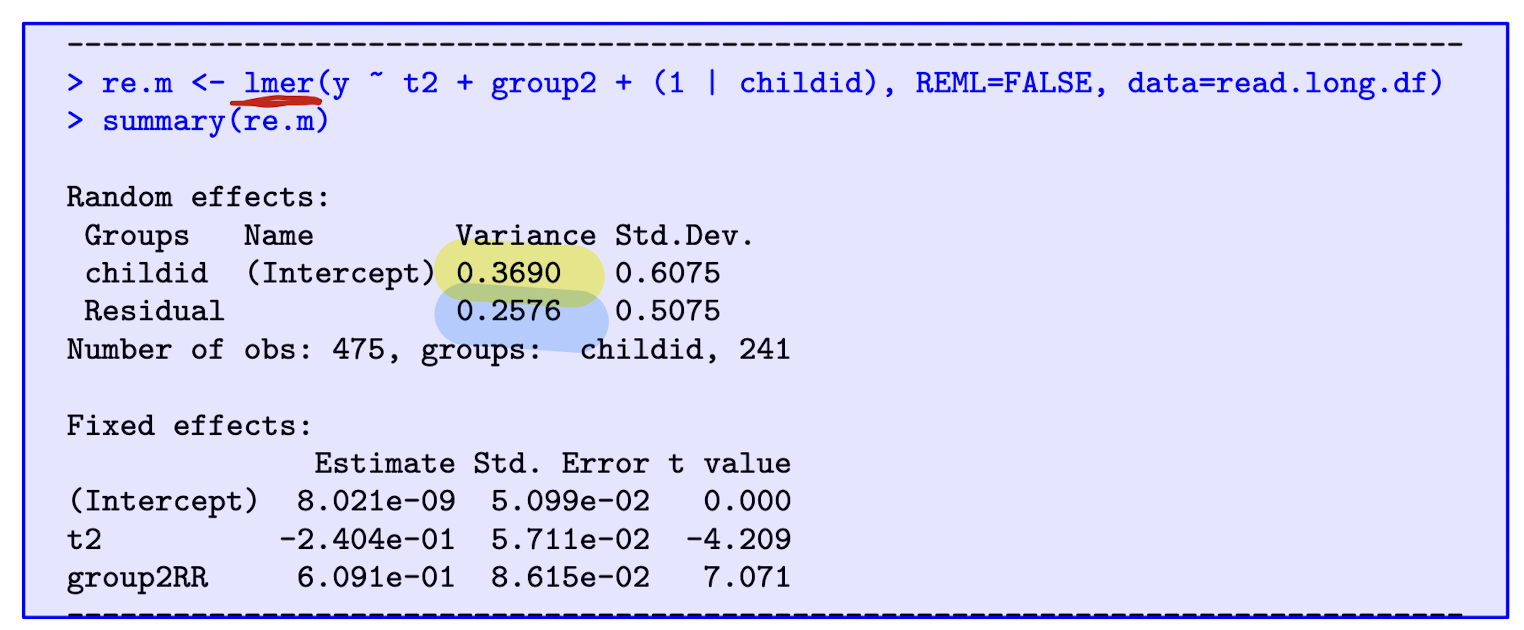
Reading Recovery: Random effects model. Interpret the effect and find \hat{\rho} .

The effect of RR estimated as 0.609, so reading recovery associated with expected increase in reading score by 0.609 points.

-

\hat{\rho} = \frac{0.3690}{0.3690 + 0.2576} = 0.59 

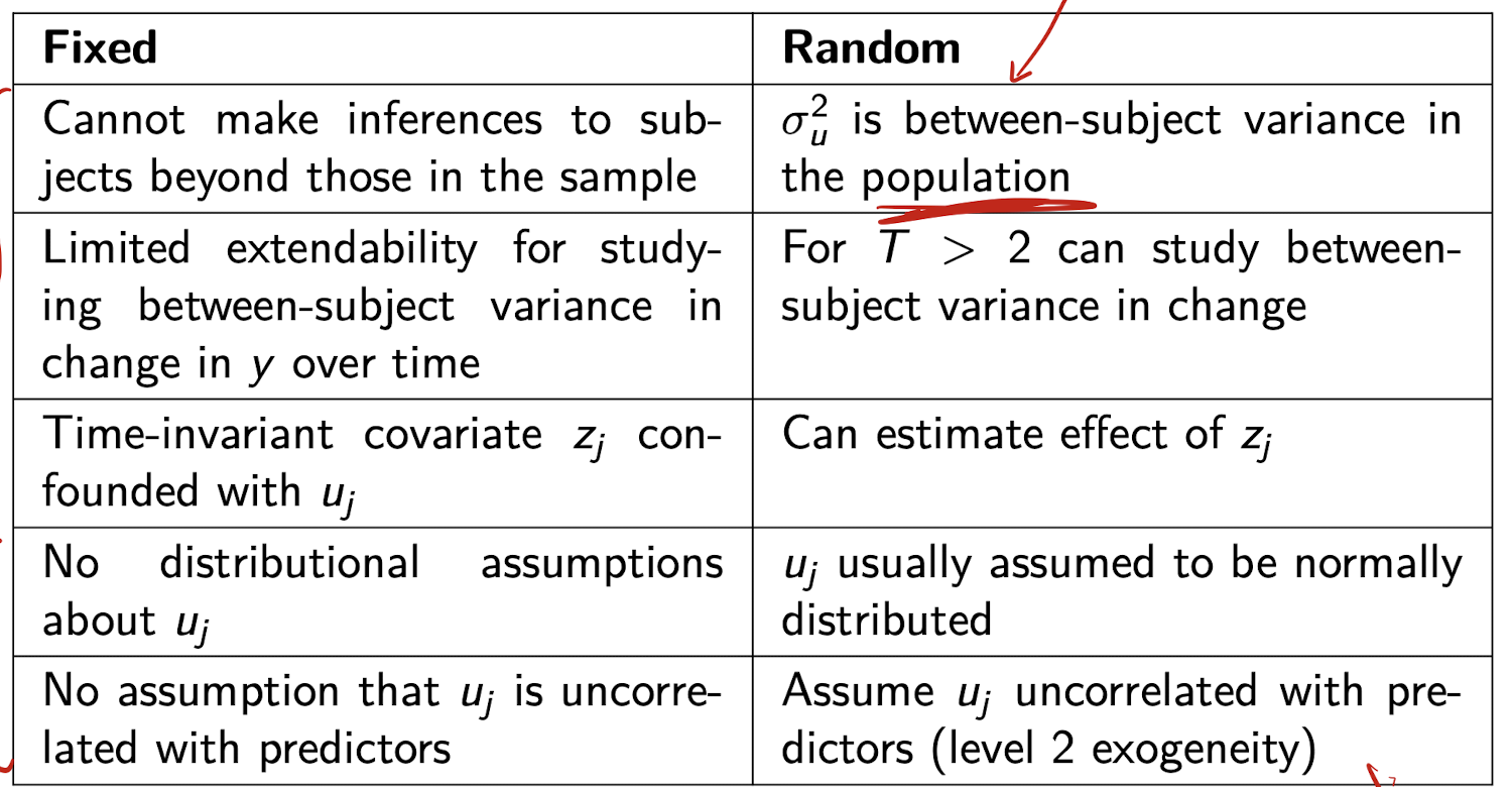
When should I use fixed effects vs. random effects?

Fixed effects (FE):

* Use when you are only interested in individuals in your sample

* No distributional assumptions about subject-specific effects (u_j)

* Allows u_j to be correlated with predictors (x_ij)

* Good for controlling for all time-invariant individual differences

Limitation: cannot estimate effects of time-invariant covariates (like z_j)

-

Random effects (RE):

* Use when you want to generalize to a broader population

* Assumes u_j ~ N(0, σ_u²) and Cov(u_j, x_ij) = 0 (level-2 exogeneity)

* More efficient than FE if assumptions hold

* Can estimate effects of time-invariant variables

* Can study between-subject variance, especially when T > 2

-

Key trade-off:

FE is more flexible and robust to correlation between u_j and x_ij

RE is more efficient, but only valid if u_j is uncorrelated with predictors

How is the fixed effects (FE) model extended when $T > 2$?

* Assume outcome y_{ij} changes linearly with time t_{ij}:

y_{ij} = \alpha_0 + \alpha_1 t_{ij} + \delta x_{ij} + u_j + e_{ij}

* Step 1: Take subject-specific means:

\bar{y}_j = \alpha_0 + \alpha_1 \bar{t}_j + \delta \bar{x}_j + u_j + \bar{e}_j

* Step 2: Subtract to eliminate u_j:

y_{ij} - \bar{y}_j = \alpha_1(t_{ij} - \bar{t}_j) + \delta(x_{ij} - \bar{x}_j) + (e_{ij} - \bar{e}_j)

-

* Interpretation:

- Removes time-invariant heterogeneity (u_j)

- Called "de-meaning"

- Can estimate \alpha_1 and \delta using OLS

What is the RE model for T > 2 and how does it compare to FE?

Model assumes linear growth in outcome:

y_{ij} = \alpha_0 + \alpha_1 t_{ij} + \delta x_{ij} + u_j + e_{ij}

u_j \sim \text{i.i.d. } N(0, \sigma_u^2)

e_{ij} \sim \text{i.i.d. } N(0, \sigma_e^2)

-

Same structure as fixed effects model, but:

- u_j is now random, not fixed

- Assumes \text{cov}(u_j, x_{ij}) = 0 (level 2 exogeneity)

y_{ij} = outcome for individual j at time i

t_{ij} = time

x_{ij} = predictor

u_j = individual-specific random effect

e_{ij} = residual error

Special case of a linear growth model

Same FE vs RE comparison applies for T > 2

How can x_{ij} be decomposed to separate within and between effects?

x_{ij} = (x_{ij} - \bar{x}_j) + \bar{x}_j

x_{ij} is the value of covariate x for person j at time i

\bar{x}_j is the average of x for person j over time

This decomposition allows us to separately estimate within- and between-person effects

What is the within-person effect \delta^W?

\delta^W is the effect of the deviation x_{ij} - \bar{x}_j on y_{ij}

This captures how changes in x over time within the same person affect the outcome

y_{ij} is the outcome for person j at time i

What is the between-person effect \delta^B?

\delta^B is the effect of \bar{x}_j on \bar{y}_j

This captures how people who differ in average x differ in their average outcomes

\bar{x}_j is the mean of x_{ij} over time for individual j

\bar{y}_j is the mean of y_{ij} over time for individual j

How are \delta^W and \delta^B handled in a fixed effects model?

Only \delta^W is identified in fixed effects models

Time-invariant components like \bar{x}_j drop out during demeaning

Between-person differences are not used in estimation

How are \delta^W and \delta^B handled in a random effects model?

The estimated \delta is a blend of \delta^W and \delta^B

We cannot separate them unless we include both x_{ij} - \bar{x}_j and \bar{x}_j as predictors

This allows \text{cov}(u_j, x_{ij}) \ne 0

What model allows separate estimation of \delta^W and \delta^B in a random effects framework?

y_{ij} = \alpha_0 + \alpha_1 t_{ij} + \delta^W (x_{ij} - \bar{x}_j) + \delta^B \bar{x}_j + u_j + e_{ij}

y_{ij} is the outcome

t_{ij} is time

u_j is the subject random effect

e_{ij} is the residual

Including both components isolates within and between effects

- GROWTH CURVE MODELS -

Types of methods for T > 2

• Growth curve models (aka latent growth/trajectory models)

• Marginal models

• Dynamic panel models

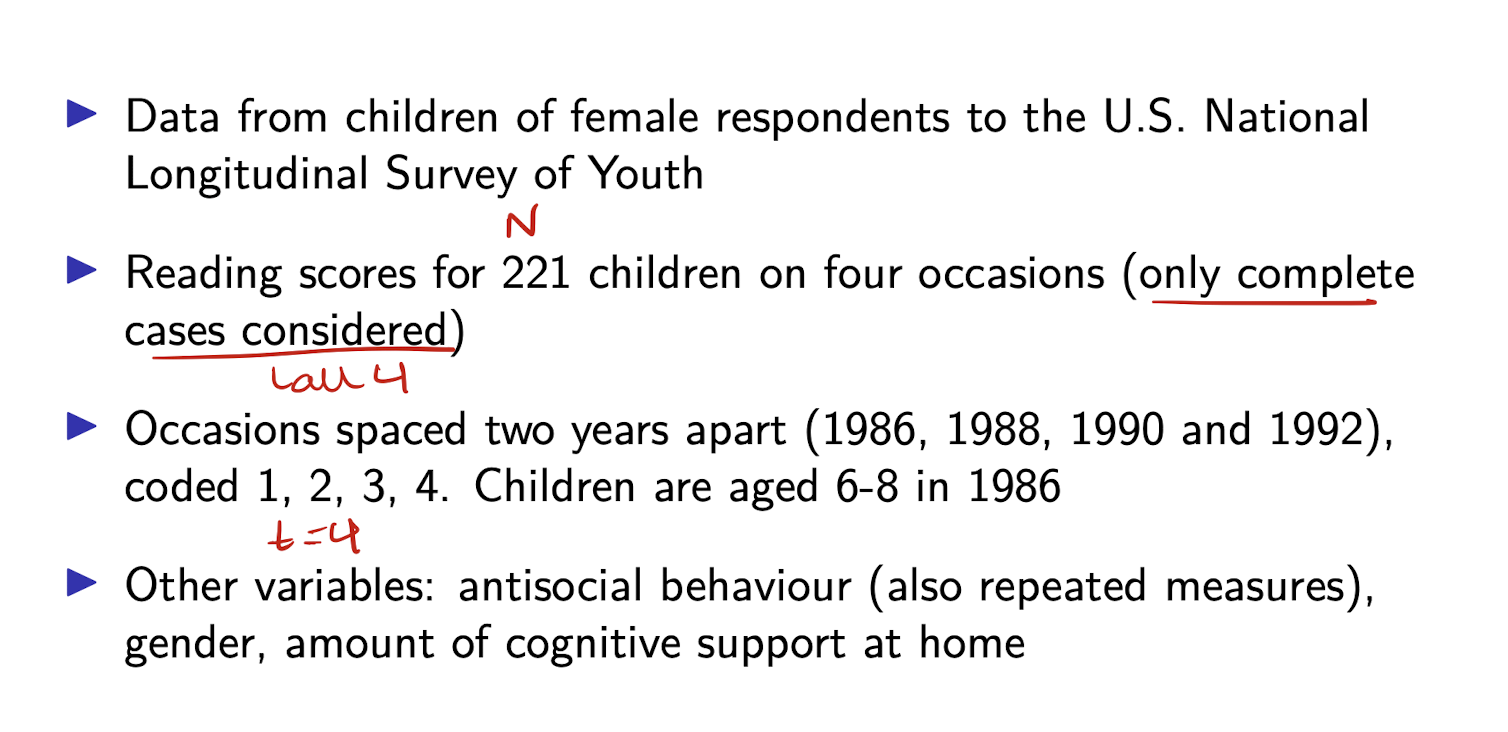
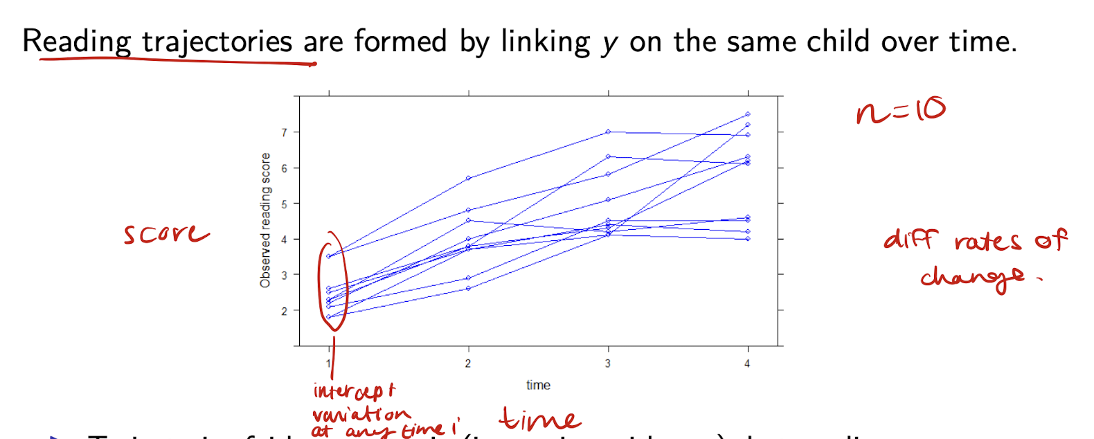
Example: reading development

Growth curve models can be viewed as what 2 types of models?

1. Multilevel models - time is treated as an explanatory variable

2. Structural equation models

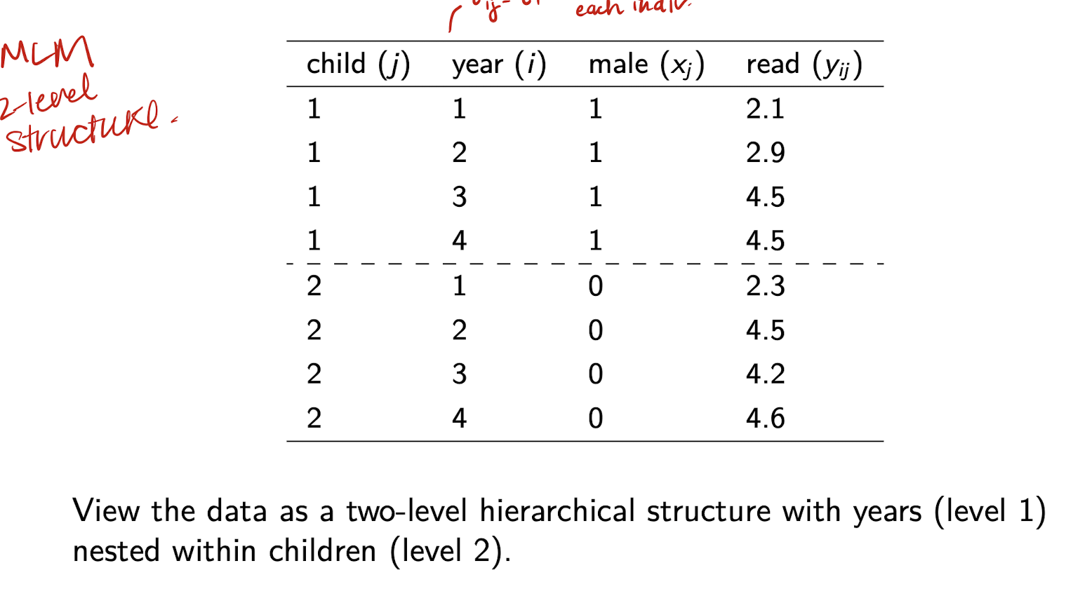
GCM as a multilevel model

Require the data to be in long form

What does GCM aim to do?

Fit a curve that captures observed variation within and between subjects as closely as possible.

Questions from reading development example:

1. What is the nature of reading development with age? (Linear/nonlinear)

2. How much do children vary in their initial reading score? In their rate of development?

3. Does the initial score and rate of change depend on covariates?

What is the basic linear growth model with random intercept? (RI Model)

y_{ij} = \beta_0 + \beta_1 t_{ij} + u_{0j} + e_{ij}

- u_{0j} is the subject-specific (random) intercept

- e_{ij} is the occasion-level residual

What does u_{0j} represent in the model y_{ij} = \beta_0 + \beta_1 t_{ij} + u_{0j} + e_{ij}?

u_{0j} represents unmeasured individual characteristics that are fixed over time

How can the random intercept model be rewritten to emphasize individual variation in intercepts?

y_{ij} = \beta_{0j} + \beta_1 t_{ij} + e_{ij}

\beta_{0j} = \beta_0 + u_{0j}

What does \beta_{0j} represent in the growth model?

\beta_{0j} is the intercept for individual j

- \beta_0 is common to all individuals

- u_{0j} is unique to individual j

What type of variation does this model allow for in y?

Individual variation in the level of y

- The rate of change \beta_1 is the same for all individuals

What are the assumptions of the basic linear growth model?

• Homoskedasticity - variation within each person across time AND between people are both fixed

• Exogeneity - The things we’re using to predict the outcome (like time and people) aren’t related to the random noise in the data.

• Distributional (when using MLE) - e’s and u’s are normal and uncorrelated

What is the homoskedasticity assumption in the basic linear growth model?

\text{var}(e_{ij} \mid t_{ij}, u_{0j}) = \text{var}(e_{ij}) = \sigma_e^2

- \text{var}(u_{0j} \mid t_{ij}) = \text{var}(u_{0j}) = \sigma_{u0}^2

- Fixed variances across individuals for level I and II

What is the exogeneity assumption in the basic linear growth model?

\text{cov}(e_{ij}, t_{ij}) = 0

- \text{cov}(u_{0j}, t_{ij}) = 0

- Similar to assuming \text{cov}(u_j, x_{ij}) = 0

What are the distributional assumptions of the basic linear growth model when using MLE?

e_{ij} \sim \text{i.i.d } N(0, \sigma_e^2)

- u_{0j} \sim \text{i.i.d } N(0, \sigma_{u0}^2)

- \text{cov}(e_{ij}, u_{0j}) = 0

- All terms are normally distributed and uncorrelated

What is the variance of y_{ij} in the random intercept model?

\text{var}(y_{ij} \mid t_{ij}) = \text{var}(u_{0j} + e_{ij}) = \sigma^2_{u0} + \sigma^2_e

What is the covariance between two observations y_{ij} and y_{i'j} for the same person?

\text{cov}(y_{ij}, y_{i'j} \mid t_{ij}, t_{i'j}) = \sigma^2_{u0} \quad (i \ne i')

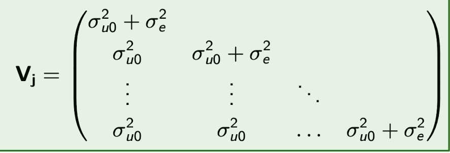
What is the implied covariance matrix \mathbf{V}_j for subject j in a random intercept model?

It is a T_j \times T_j matrix with:

- \sigma^2_{u0} + \sigma^2_e on the diagonal

- \sigma^2_{u0} on the off-diagonals

What is the N x N covariance matrix \mathbf{V} for all subjects j ?

What is intra-individual correlation \rho in a random intercept model?

It measures how strongly two observations from the same person are correlated

- Also called the variance partition coefficient

It tells us how much of the total variance is due to differences between individuals

- Higher \rho means more of the variance is between-person rather than within-person

What is the formula for intra-individual correlation \rho?

\rho = \text{corr}(y_{ij}, y_{i'j} \mid t_{ij}, t_{i'j}) = \frac{\sigma^2_{u0}}{\sigma^2_{u0} + \sigma^2_e} \quad (i \ne i')