The Closed Economy Three Equation Model

How is the dynamic IS curve derived?

• Consumption and investment functions are substituted into the GDP identity

• Y^D = C + I + G = c₀ + c₁(1 - t)y + a₀ - a₁r + G

• Impose the equilibrium condition, output = expenditure

• y = 1/(1 - c₁(1 - t)) (c₀ + a₀ + G - a₁r) = k(c₀ + a₀ + G) + ka₁r = A - ar

• This represents goods market equilibrium (demand = supply)

What does A - ar describe?

• This describes output as a multiple of exogenous spending decisions, adjusted for the negative effect of higher interest rates on investment

The slope and constants of the IS curve

• y = A - ar, where the inverse relationship between output and investment can be plotted in r-y space, r = A/a - (1/a)y

• a = ka₁, where k is the multiplier, where 0 < k < 1, 0 < t < 1, and real interest elasticity of investment a₁ > 0 (how much investment changes w.r.t real interest rate)

• Thus a > 0, so in the IS curve where -ar exists, the slope is negative

• The exogenous component, A = k(c₀ + a₀ + G) involves (via k) the MPC, the marginal tax rate, autonomous consumption, autonomous investment, and government spending

What are the three expenditure components?

• c = 𝑐₀ + 𝑐₁(1 − 𝑡)𝑦 is Real consumer spending, whose equation makes clear is assumed to not depend on 𝑟

• 𝐼 = 𝑎₀ −𝑎₁𝑟 is Real business investment, which depends on 𝑟

• 𝐺 is Government consumption/spending, which is assumed to not depend on r

What are properties of the IS curve?

• Downwards sloping meaning that high r means low y and low r means high y

• A higher multiplier means that the slope becomes flatter and vice versa (the multiplier, 1/(1-c₁(1-t)) increases via lower t or higher c₁)

• An increase in investment sensitivity to interest rates, a₁, flattens the slope

What shifts the IS curve?

• Any change in its exogenous components, c₀, a₀ or G

• The change in income resulting from these expenditure changes is given by the change in spending multiplied by the multiplier

Lag in the IS curve and the monetary policy transmission mechanism

• Typically, the curve avoids time-specific subscript to emphasise the general formula, but the dynamic curve is written as y_t = A - ar_{t - 1}

• CB sets an interest rate which is mediated through financial markets, affecting things like the exchange rate and asset prices before reaching the real economy in the labour market and in domestic prices

Properties of the Phillips Curve

• The output gap is negatively related to unemployment

• There is a positive relation between inflation and the output gap

• Downwards-sloping in π-u space, upwards-sloping in π-r space

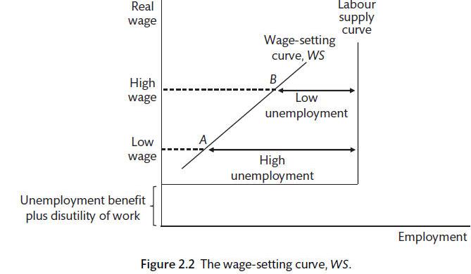
Properties of wage-setting curve

• In equilibrium the market normally doesn’t clear, resulting in some unemployment because firms pay efficiency wages above a worker’s reservation wage to induce them to work hard

• At high levels of unemployment, a low wage is needed, and vice versa

• A positive output gap (rise in output) reduces unemployment, reducing cost of job loss therefore requiring higher wages

Supply shocks in the closed economy model

• These are only caused by shifts in the wage-setting or price-setting curves; understanding the models which motivate the Phillips curve are therefore crucial

Writing the Wage-setting curve

• w^WS = W/p^E = f(N, z_W), where z_W captures all the factors that might influence wage-pushes besides the natural rate of employment (like union power, increased bargaining etc)

• w^WS = W/p^E = α(y_t - y_e) + z_W is another way of writing it, because wages and inflation are positively correlated

• B is included in z_W, where B is a constant which represents the pecuniary and non-pecuniary benefits of not working including disutility from work (unemployment benefits)

What shifts the wage-setting curve down (supply shock)?

• Fall in unemployment benefits (amount, duration, increase in application difficulty or tougher eligibility criteria)

• Improvement in working conditions (reduction in net disutility of work)

• More/cheaper monitoring of work effort; lower cost of firing shirkers

• Unions have less bargaining power or legal protection leading to less union nominal markup

• These allow for higher costs of unemployment and lower efficiency wages to be paid

Wage inflation in the WS curve

• Taking logs of W/p^E = α(y_t - y_e) + z_W, derive (ΔW/W)_t = (ΔP^E/P^E)_{t - 1} + α(y_t - y_e)

  • Expected wage inflation is equal to expected inflation + economic activity pressures, assuming P^E = P_{t - 1}

• Therefore, the higher expected inflation is, the higher nominal wage growth will be

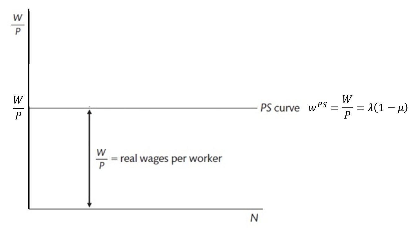
Properties of the price-setting curve

• Price changes depend positively on wage increases, negatively on productivity decreases, and assuming markup is fixed, not on the market

Writing the Price-Setting curve

• Prices depend on marginal costs, which is the nominal wage per unit of output, W/λ, as well as the markup, μ, which measures the extent to which prices exceed unit labour costs in percentage points

  • Very simple production function; labour is the only input (no capital)

• P = (1 + μ) W/λ

• w^PS = λf(μ, Z_p)

• Rearrange to get W^PS = W/P = 1/(1 + μ)λ ≈ λ(1 - μ)

  • This allows us to put it in W/P - N (Real wage - Employment) space

• Could be conversely understood as a function of markup and price-push factors, W^PS = λf(μ, z_p)

Graphical interpretation of the PS curve

• A horizontal PS curve occurs if marginal productivity of labour is constant (ie, = average product of labour)

• Vertical distance between the PS curve and the horizontal axis are real wages per worker

• If λ is higher on the than the real wage, the vertical distance between the lines is the real profit per worker (μλ)

What causes shifts in the Price-Setting curve?

• Because it is drawn in real wage-employment space, upwards price pushes will shift the PS curve downwards because it’s in the denominator of the y-axis, W/P

• A rise in the tax wedge shifts PS down (tax wedge = real consumption wage minus real product wage, increase in taxes on labour which is shifted onto consumers), a rise in markup and a fall in productivity shift the curve downwards, pushing prices up

Price changes modelled in the PS curve

• P = (1 + μ) W/λ

• Taking logs, logP = log(1 + μ) + logW - logλ

• Differentiating, assume μ is constant, dlogP/dt = dlogW/dt - dlogλ/dt

• = 1/P · dP/dt = 1/W · dW/dt - 1/λ · dλ/dt = ΔP/P = ΔW/W - Δλ/λ

• Such that price growth = wage growth - productivity growth

• When productivity of labour is a constant, a change in wages is equal to the change in prices

Combining the wage-setting and price-setting curves to create the Phillips Curve

• Wage-inflation: (ΔW/W)_t = (ΔP^E/P^E)_{t - 1} + α(y_t - y_e)

• Price-inflation: (ΔP/P)_t = (ΔW/W)_t - (Δλ/λ)_t

• Wage-setters set wages in accordance with last periods price inflation, to which price-setters respond by changing their price to ensure their markup remains fixed

• Assuming there are no changes in productivity, prices rise in line with wage increases/demands

• Substituting wage-inflation into price-inflation, we get:

  • (ΔP/P)_t = (ΔP^E/P^E)_{t - 1} + α(y_t - y_e), where there is no productivity variable because it’s assumed to be 0

    • This can be simplified as π_t = π_{t - 1} + α(y_t - y_e)

Graphical understanding of the Phillips Curve

• In inflation-output space

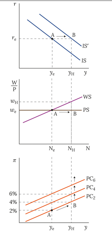
• A positive AD shock shifts the PC upwards increasing employment and worker bargaining power, meaning a wage-setter chooses a higher nominal wage to cover the output gap (higher on the WS-curve)

• Price-setters respond by increasing prices to cover higher nominal wage costs, keeping real wages constant

A positive AD shock without policy response in the current model

• The IS curve shifts rightwards, intersecting the wage setting curve at a higher nominal value and causing an upwards shift in the Phillips Curve

What assumptions can influence inflation expectations?

• The general form might be characterised as π_t = π^E + α(y_t - y_e)

• Adaptive expectations: π_t = π_{t - 1} + α(y_t - y_e)

• Anchored expectations: π_t = π^T + α(y_t - y_e), where π^T is inflation targeted by the CB

The Inverted Phillips Curve

• In terms of output rather than inflation, with an ‘inflation gap’ existent

• y_t = y_e + 1/α · (π_t - π^E)

• The Phillips Curve is the constraint the CB has to operate with when optimising its choice of inflation and output

Graphic interpretation of the WS curve

• Real wage, W/P on the y-axis, Employment on the x-axis

• Labour-force = Natural rate of employed + Unemployed, L = N + U; unemployed is just ‘structural’ or ‘frictional’ which exists regardless of demand

• Labour supply curve is an inverted L-shape (perfectly competitive, typically just vertical)

  • Vertical at ‘full employment’, horizontal is the opportunity cost of working (reservation wage = unemployment benefit + net nonpecuniary disutility of work)

    • It is assumed that everyone’s disutility of work is the same

• Wage-setting curve is effectively a labour supply curve under imperfect conditions (like efficiency wages, bargaining power imperfections)

• Non-intersection of WS and Labour Supply implies a level of employment above structural unemployment due to efficiency wages

Demand shocks in the Wage-Setting Curve

• A demand shock is effectively an output shock, meaning a rise in income and a positive output gap; the rise in income is correlated with a rise in employment

• There is a reduced cost of job loss meaning a higher wage is required to incentivise workers putting upwards pressure on nominal wages; unions can only demand a higher nominal wage because they don’t control prices

Type of costs incurred in periods of inflation

• Shoe-leather costs: The costs incurred by holding cash during inflationary periods and needing to spend more time managing one’s financial assets

• Menu costs: The costs incurred on businesses when they must frequently review and update their prices (as in literally changing prices on a menu)

Why is low-level inflation targeted?

• To ‘oil the wheels’ of the labour market; it allows firms the flexibility to make real wage reductions without changing the nominal value, thus avoiding frustration generated by apparent wage-change

What does the MR (monetary rule) curve show?

• It shows the chosen output gap (inflation level) of the central bank for any shock; it shows the path along which the CB tries to guide inflation levels back to target

Deriving the MR curve graphically

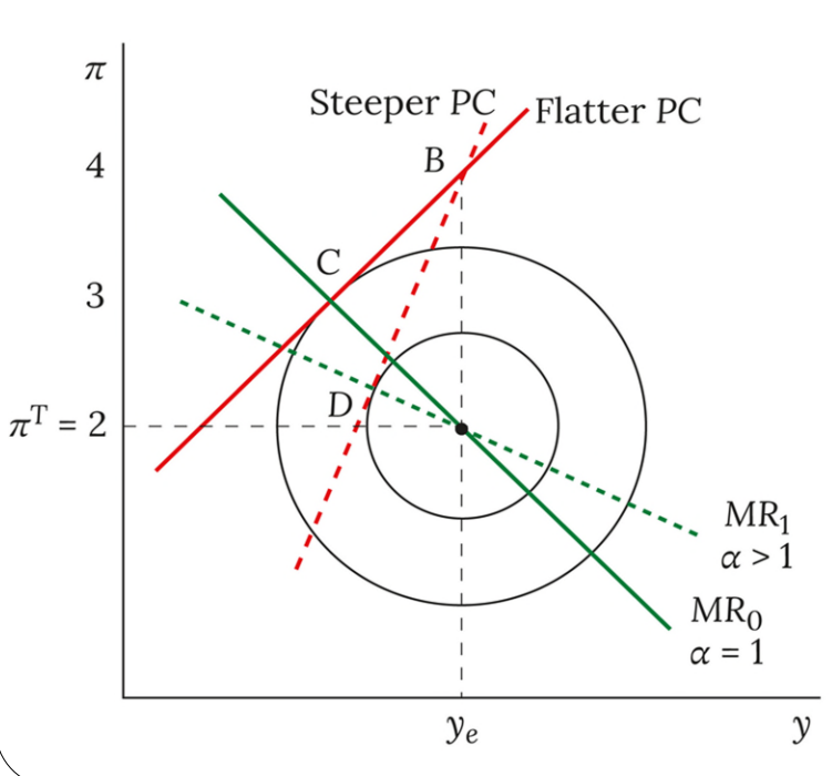
• Define CB utility in a Loss function, L = (y_t - y_e)² + β(π_t - π^T)², where β is the relative weight attached to inflation; a higher β characterises a more inflation-averse CB

• The Phillips curve acts as a constraint on what employment-inflation level a CB can choose, with many Phillips curves intersecting the Loss function, representing different levels of target inflation; where π_t = π^T, it pass through the bliss point at the centre of the loss function

• The MR curve is derived by identifying and joining the tangency points between the Phillips curves and the loss function

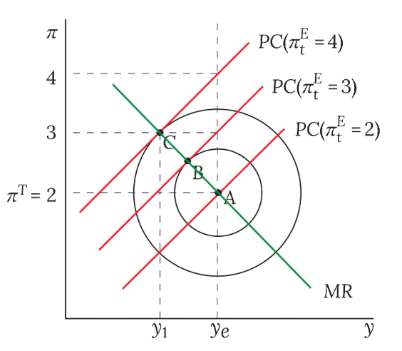
Graphical interpretation of the loss function

• A β>1 means inflation averse, meaning that the loss circles will be squat to account for a smaller range of inflation deviation, whereas unemployment averse will be taller and skinny to allow for less unemployment deviation

Writing the MR curve

• (y_t - y_e) = -αβ(π_t - π^T)

• This is different from a Taylor rule because it expresses a policy response in terms of choosing an output gap rather than choosing an interest rate

Deriving the MR curve mathematically

• Minimise, L = (y_t - y_e)² + β(π_t - π^T)², subject to the Phillips curve constraint, π_t = π_{t - 1} + α(y_t - y_e) with respect to y_t

• Obtain (y_t - y_e) = -αβ(π_t - π^T)

The effect of anchored expectations

• When there is a temporary demand shock, inflation will readjust and no policy response is required; expectations are less anchored as the shock is more sustained

• A permanent demand shock leads to a shift in the IS curve

The deflation trap

• Fisher equation, i = r + π^E

• There is a zero lower nominal bound on interest rates, meaning sometimes the CB can’t set a rate low enough to combat deflation

• Thus, deflation continues and expectations don’t improve, causing a trap; we must resort to fiscal policy or quantitative easing to mitigate the problem

The Fisher equation and finding the policy rate

• r_t^E = i_t - π^E_{t + 1} with adaptive expectations, then the inflation rate of the next period is just expected to be the inflation rate of the current period, π_t

Forecasting the IS curve

• Since the IS curve components target output in the next period, y_t+1 = A_t+1 - ar_t, current interest rates are not linked to current output

• Thus, the CB must set the nominal interest rate to achieve the real interest rate which they forecast will generate their preferred output gap

  • It is central to recognise that there is a lack in the transmission mechanism of monetary policy

How sensitivity parameters affect policy response

• Both α and β affect the MR curve; if either of them is higher (sensitivity to the output gap and inflation respectively) then the MR curve will be flatter

• Reiterating, β>1 leads to a higher compensatory output reduction after an inflation shock

• A higher α (steeper PC) means inflation is more responsive to output, so cutting output decreases inflation by more

• If β>1 then the CB is more inflation averse, leading to a flatter MR curve (in line with the more squat iso-loss curves, which involves a sharper cut in output to response to a shock)

Slopes in the TEM

Components influencing policy response

• π_t: shifts the MR curve

• y_e: shifts the MR curve

• β: sensitivity to inflation deviations, affects the iso-loss curve shapes and slope of MR

• α: sensitivity to output gap deviation, affects PC and MR slopes

• a: interest sensitivity of investment, alters IS slope

Stabilisation Policy in the TEM

• After an inflation shock, the PC shifts up to a new place on the PC

• CB forecasts the PC for the next period and picks the optimal point on it (where it intersects the MR curve) which decides the interest rate it must adopt to move the economy back to the equilibrium level

Impulse response functions

• On the y-axis is value of the variable and on the x-axis is time, to measure how the variable changes with respect to time

• Use them whenever using the TEM to show understanding of how the variables change over time

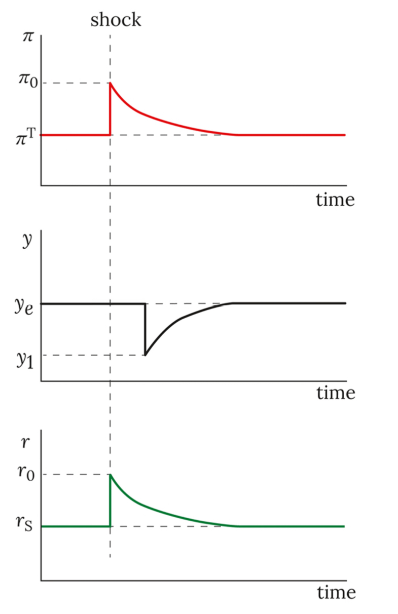
Effect of a permanent demand shock

• In the absence of a policy response, inflation expectations remain high leading to increasing inflation

• The IS curve shifts and thus the PC also moves up continually unless the CB changes AD by altering the interest rate

• Even after all the interest changes, we return to equilibrium output and inflation, but we never return to the initial real interest rate which is increased permanently