OMIS 327

Quantitative Analysis

scientific approach to managerial decision making

Business analytics

 data driven approach to decision making that allows companies to make better decisions. 

3 categories of business analytics

1. Descriptive - study and consolidation of historical data for a business and industry to measure how it is performing

2. Predictive - aimed at forecasting future outcomes based on patterns in the past data 

3. Prescriptive - involves the use of optimization methods to provide new and better ways to operate

Quantitative Analysis Approach (QAA)-

 scientific approach to managerial decision making in which raw data are processed and manipulated to produce meaningful information.

Steps to QAA - 

1. Develop a clear, concise statement of the problem

   1. Must be specific and measurable objectives 

2. Develop a model (model = mathematical representation of a situation)

   1. Model = realistic, solvable, and understandable mathematical representations of a situation. 

   2. Controllable inputs = decision variables

   3. Uncontrollable inputs = pareteres; things outside of their control. 

   4. Deterministic models = a of the values used in the model are known with complete certainty

   5. Probabilistic models = variables used in the model are estimates based on probabilities. 

3. Acquiring input data

   1. GIGO Rule - input data must be accurate. 

   2. Can come from a variety of sources

4. Developing a solution 

   1. Manipulating the model to arrive at the best (optimal solution)

   2. Ex: solving equations, trial and error, complete enumeration (trying all [possible values.)

5. Testing the solution

   1. Both input data and the model should be tested for accuracy and completeness before analysis and implementation. 

6. Analyzing the results and sensitivity analysis 

   1. Determining the implications of of the solution

   2. Sensitivity analysis - postoptimality analysis determines how much the results will change if the model or input data changes. 

7. Implementing the results

   1. Incorporates the solution into the company

   2. Change takes place over time, so even successful implementations must be monitored to determine if modifications are necessary

Mathematical model-

set of mathematical relationships, expressed in equations and inequalities

Variable

a measurable quantity that may vary or is subject to change, can be controllable or uncontrollable

Parameter

a measurable quantity that is inherent in the problem

Profit

= revenue - (fixed cost + variable cost) 

= (selling price per unit) (number of units sold) 

= sX - [f + vX]

S = selling price price per unit

f = fixed cost 

v = variable cost per unit 

X = number of units sold

Advantages of mathematical modeling 

1. Models can accurately represent reality 

2. Models can help a decision maker formulate problems

3. Models can give us insight and information 

4. Models can save time and money in decision making and problem solving

5. A model may be the only way to solve some large or complex problems in a timely fashion 

6. A model can be used to communicate problems and solutions to others

Possible problems in quantitative analysis approach 

• Defining the problem

  • Conflicting viewpoints

  • Impact on other departments

  • Beginning assumptions

  • Solutions outdated

• Developing a model

• Acquiring input data 

• Developing a solution

• Testing the solution

• Analyzing teh results

6 steps in decision making 

1. Clearly define the problem at hand 

2. List the possible alternatives

3. Identify the possible outcomes or states of nature

4. List the payoff (typically profit) of each combination of alternatives and outcomes

5. Select one of the mathematical decision theory models

6. Apply the model and make your decision

Types of decision making environments 

• Decision making under certainty - decision maker knows with certainty the consequences of every alternative or decision choice 

• Decision making under uncertainty - the decision maker does not know the probabilities of the various outcomes

• Decision making under risk - there are several possible outcomes for each alternative, and the decision maker knows the probability of occurrence of each outcome.

Decision making under uncertainty criteria

1. maximax - find maximum max

2. maximin - find the maximum of all minimum

3. minimax regret -  (calculated by column vertically not horizontally by row) 

• Then pick smallest minimax by row (want the least regret)

• difference between the optimal profit and the actual payoff for a decision

Decision making under risk criteria 

• Selecting the alternative with the highest expected monetary value 

5 Steps of Decision Tree Analysis 

1. Define the problem 

2. Structure or draw the decision tree

3. Assign probabilities to the states of nature

4. Estimate payoffs for each possible combination of alternatives of nature

5. Solve the problem by compound EMVs for each state of nature node. This is done by working backwards, that is, starting at the right of the tree and working back to the decision nodes on the left. Also at each decision node, the alternative with the best EMV is selected.

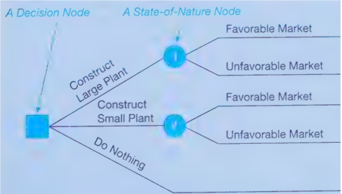
All decision trees contain 

• Decision nodes - one of several alternatives may be chosen

• Decision points

• State of nature nodes - out of which one state of nature will occur 

• State of nature points

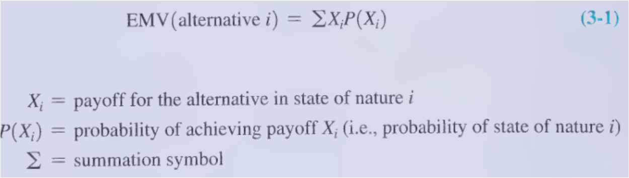
Expected monetary value (EMV)

long run average value of that decision. The sum of possible payoffs of the alternative, each weighted by the probability of that payoff occurring 

EMV (alternative i)

= ΣX_iP(X_i)

X_i  = payoff for the alternative in state of nature i

P(X_i) = probability of achieving payoff X_i (i.e., probability of state of nature i) 

Σ = summation symbol 

Expected value with perfect information (EVwPI) =

Σ(Best payoff in state of nature 7 i) (probability of state of nature 7 i)

EPVI

= expected value of perfect information

• EVwPI — Best EMV

Expected value of sample information (EVSI)

 increase in expected value resulting from the sampling information. 

 = (EV with SI + cost) — (EV without SI)

Efficiency of sample information =

 (EVSI/ EVPI)100%

Business Analytics

 a data driven approach to decision making

Profit Function (px) =

revenue - total cost 

Expected opportunity loss (EOL)

Σ(opportunity loss)*(probability) 

Decision alternatives

different possible strategies the decision maker can employ

States of nature

refer to future events, not under the control of the decision maker, which may occur. 

• States of nature should be defined so that they are mutually exclusive and collectively exhaustive

Payoff

consequence resulting from a specific combination of a decision alternative and a state of nature

Linear programming (LP) is a widely used

mathematical modeling technique designed to help managers in planning and decision making relative to resource allocation.

Requirements of Linear programming 

1. Problems seek to maximize or minimize an objective

2. Constraints limit the degree to which the objective can be obtained

3. There must be alternatives available

4. Mathematical relationships are linear

Properties of linear programs

1. One objective function 

2. One or more constraints 

3. Alternative courses of action

4. Objective function and constraints are linear—proportionality and divisibility

5. Certainty 

6. Divisibility 

7. Nonnegative variables

The steps in formulating a linear program follow:

1. Completely understand the managerial problem being faced. 

2. Identify the objective and the constraints.

3. Define the decision variables.

4. Use the decision variables to write mathematical expressions for the objective function and the constraints.

Slack

 (Amount of resource available) — (Amount of resource used)

Surplus

(Actual amount) — (Minimum amount)

Maximax (optimistic) criteria

• find the maximum payoff for each alternative, pick the maximum out of the list of maximum 

• Locate the maximum payoff for each alternative

• Select the alternative with the maximum number

When there are several possible states of nature and

the probabilities associated with each possible state are known

• Most popular method - choose the alternative with the highest expected monetary value (EMV) similar to expected value

• For each alternative the emv is calculated by

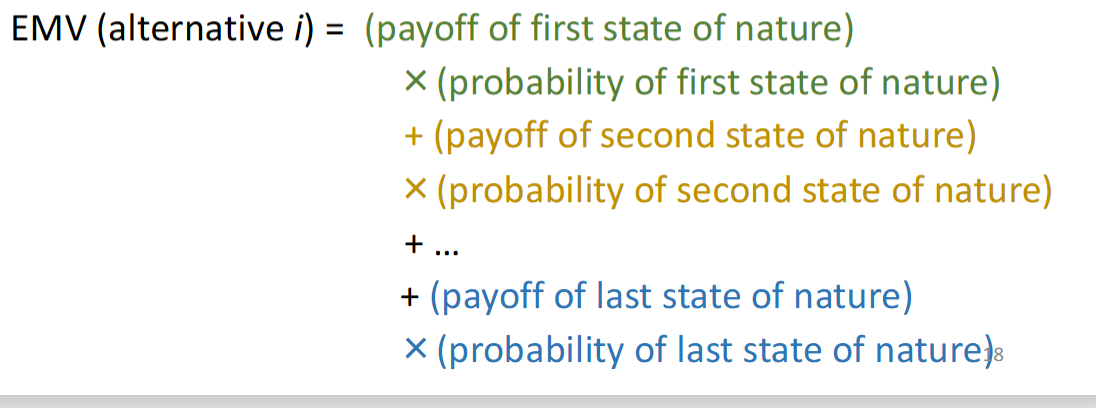
 EMV definition

 ( Expected Monetary Value) A higher, positive EMV signifies a more profitable, lower-risk decision or investment.

Minimax regret

 Best payoff in each state – (x individual payoff of alternative)

•  (calculated by column vertically not horizontally by row) 

• Then pick smallest minimax by row (want the least regret)

• Difference between the optimal profit and the actual payoff for a decision

How to solve for minimax regret 

• Calculate opportunity loss by subtracting each payoff in the column from the best payoff in the column (i.e. under each state of nature)

• Find the maximum opportunity loss for each alternative and pick the alternative with the minimum number.

Optimization (mathematical) model includes: 

Objective function - mathematical expression that describes the problems objective, such as maximizing profit or minimizing cost

Constraints - a set of restrictions or limitations, such as production capacities 

Uncontrollable inputs - factors that are not under the control of the decision maker

Decision variables - controllable inputs, decision alternatives specified by the decision maker, such as the number of units of a product to produce

Linear programming problem -

 both the objective function and the constraints are linear

• Functions in which each variable appears in a separate term (ex: +, -, , *) raised to the first power and is multiplied by a constant (which could be 0) 

• Separate term -> x + y good, xy bad, x/y bad 

• Nonlinear format = bad (ex: √z) (ex: x^-1)

• Its okay to have a single variable ex: 1 + x

Linear constraints

 linear functions that are restricted to be “≥”, “=”, “≤” or a constant

Nonnegativity constraint

 X, Y ≥ 0

*basically just saying that your answer can’t be negative

Algebraic model

 AX + BY ≤ 0

Ex: 20x + 30y  ≤ 0 

Linear constraint note-

usually (but not always) the linear function is on the left hand side of a constraint, and a constant on the right hand side

Hint phrases for linear constraint 

>= constraint : at least, no less than , minimum requirement, etc

< = constraint: at most, no more than, maximum requirement, availability, capacity, budget etc

 

=  constraint = exactly, equal to etc

Maximin

(pessimistic) - find all the minimums, find the largest minimum out of all mins 

(find the max minimum) 

Linear functions cannot have

variables multiplied together or raised to powers.

Limitations of LP

forces the decision maker to state one objective only 

Integer programming

 model that has constraints and an objective function identical to that formulated by the LP. (Only difference is that one or more of the decision variables has to take on an integer value in the final solution).

3 Types of integer programming problems

1. Pure integer programming problems - cases in which all variables are required to have integer values

2. Mixed integer programming problems - cases in which some, but not all, of the decision variables are required to have integer values 

3. Zero-one integer programming problems - special cases in which all decision variables must have integer solution values of 0 or 1

Steps for integer programming 

1. Defining the problem

2. Developing a model

3. Acquiring input data

4. Testing the solution

5. Analyzing the results

6. Implementing the results

Binary variable

 0-1 decision; 0 if the condition is not met and 1 if the condition is met

In order for a break-even quantity to exist in the presence of positive fixed costs, sales price must

exceed variable cost per unit

a controllable variable is also called a:

a. decision variable.

b. mathematical model.

c. parameter.

d. measurable quantity.

a. decision variable.

A optimistic decision-making criterion is

a. decision making under certainty

b. maximax

c. maximin

d. equally likely.

b. maximax

Which of the following is not one of the steps in the quantitative analysis approach?

a. Defining the Problem

b. Observing a Hypothesis

c. Developing a Solution

d. Testing a Solution

b. Observing a Hypothesis

To be linear

 all variables should be in separate terms and only raised to the power of 1.

An objective function is required for

any optimization problem, maximization or minimization.

In an LP problem

 both objective function and constraints must both be linear.

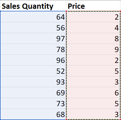
=SUMPRODUCT

multiplies 2 categories of rows (arrays) against each other

So 64 x 2, 56 x 4 etc. Need to have same number of values for both arrays so everyone gets multiplied against something

Slack

any unused resource of r an =<

Slack equation

 (Any amount of resource available) -( amount of resource used)

Binding constraints

constraints with zero slack or surplus, meaning these constraints are binding at the optimality (bottleneck constraint we need to look out for)

Nonbinding constraints

constraints with non-zero slack or surplus

General build of constraint equation 

• Functional (actual amt) on the left side 

• Constant (max / min) on the right side

  • Ex: 5x + 7y ≤ 30

Surplus

excess amount for a  >= constraint.

Surplus equation

(actual amt) - (minimum amt) 

Sensitivity analysis

(aka post optimality analysis) used to determine how the optimal solution is affected by changes (w/ specific ranges in:) (used for dynamic changes)

• Objective function coefficients

• Right hand side (RHS) values in the constraints