Year 12 WACE Maths Apps Unit 3 Flashcards 2025

Bivariate Data:

Association:

Association

Association is a general term used to describe the relationship between two (or more) variables. For example, is there an association between attitude to capital punishment (agree with, no opinion, disagree with) and gender (male, female)? Is there an association between a person’s height and foot length? The term association is often used interchangeably with the term correlation. The latter tends to be used when referring to the strength of a linear relationship between two numerical variables.

Bivariate Data:

Causation:

Causation

A relationship between an explanatory and a response variable is said to be causal if the change in the explanatory variable actually causes a change in the response variable. Simply knowing that two variables are associated, no matter how strongly, is not sufficient evidence by itself to conclude that the two variables are causally related.

Possible explanations for an observed association between an explanatory and a response variable include:

• the explanatory variable is actually causing a change in the response variable

• there may be causation, but the change may also be caused by one or more uncontrolled variables whose effects cannot be disentangled from the effect of the response variable; this is known as confounding

• there is no causation; the association is explained by at least one other variable that is associated with both the explanatory and the response variable; this is known as a common response

• the response variable is actually causing a change in the explanatory variable

Bivariate Data:

Coefficient of Determination:

Coefficient of determination

In a linear model between two variables, the coefficient of determination () is the proportion of the total variation that can be explained by the linear relationship existing between the two variables, usually expressed as a percentage. For two variables only, the coefficient of determination is numerically equal to the square of the correlation coefficient ().

Example

A study finds that the correlation between the heart weight and body weight of a sample of mice is  = 0.765. The coefficient of determination =  = 0.765² = 0.5852 … or approximately 59%.

From this information, it can be concluded that approximately 59% of the variation in heart weights of these mice can be explained by the variation in their body weights.

Note: The coefficient of determination has a more general and more important meaning in considering relationships between more than two variables, but this is not a school-level topic.

Bivariate Data:

Correlation:

Correlation

Correlation is a measure of the strength of the linear relationship between two variables. See also Association.

Bivariate Data:

Correlation Coefficient:

Correlation coefficient ®

The correlation coefficient (r) is a measure of the strength of the linear relationship between a pair of variables . Calculating  may be performed using appropriate technology.

Bivariate Data:

Explanatory Variable:

Explanatory variable

When investigating relationships in bivariate data, the explanatory variable is the variable used to explain or predict a difference in the response variable.

For example, when investigating the relationship between the temperature of a loaf of bread and the time it has spent in a hot oven, temperature is the response variable and time is the explanatory variable

It is plotted on the x-axis

Bivariate Data:

Extrapolation:

Extrapolation:

In the context of fitting a linear relationship between two variables, extrapolation occurs when the fitted model is used to make predictions using values of the explanatory variable that are outside the range of the original data.

Bivariate Data:

Interpolation:

Interpolation

In the context of fitting a linear relationship between two variables, interpolation occurs when the fitted model is used to make predictions using values of the explanatory variable that lie within the range of the original data. See also extrapolation

Bivariate Data:

Least Squares Line:

Least-squares line

In fitting a straight-line  to the relationship between a response variable  and an explanatory variable , the least‐squares line is the line for which the sum of the squared residuals is the smallest.

Determination of the equation for the least-squares line may be accessed via the use of appropriate technology.

Bivariate Data:

Residual Values:

Residual values

The difference between the observed value and the value predicted by a statistical model, for example, by a least-squares line.

Bivariate Data:

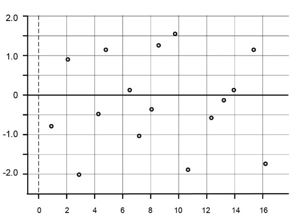
Residual Plot:

Residual plot

A residual plot is a scatterplot with the residual values shown on the vertical axis and the explanatory variable shown on the horizontal axis. Residual plots are useful in assessing the fit of the statistical model (for example, by a least-squares line).

 

When the least-squares line captures the overall relationship between the response variable  and the explanatory variable , the residual plot will have no clear pattern (be random) – see above. This is what is hoped for. If the least-squares line fails to capture the overall relationship between a response variable and an explanatory variable, a residual plot will reveal a pattern in the residuals. A residual plot will also reveal any outliers that may call into question the use of a least-squares line to describe the relationship.

Bivariate Data:

Response Variable:

In bivariate data, the response variable (also known as the dependent variable) is the variable you are trying to predict or explain. It is affected by changes in the explanatory variable (independent variable).

It is plotted on the y-axis

Bivariate Data:

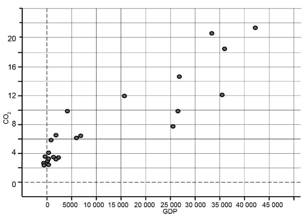
A Scatterplot:

Scatterplot

A scatterplot is a two-dimensional data plot using Cartesian co-ordinates to display the values of two variables in a bivariate data set.

For example, the scatterplot below displays the CO₂ emissions in tonnes per person (CO₂) plotted against Gross Domestic Product per person in $US (GDP) for a sample of 24 countries in 2004. In constructing this scatterplot, GDP has been used as the explanatory variable.

Bivariate Data:

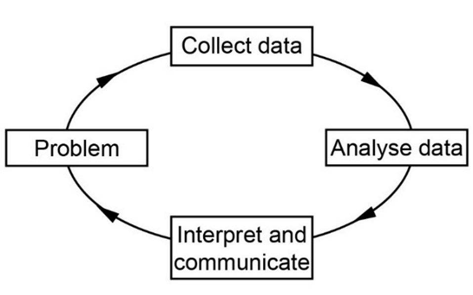
The Statistical Investigation Process:

Statistical investigation process

The statistical investigation process is a cyclical process that begins with the need to solve a real-world problem and aims to reflect the way statisticians work. One description of the statistical investigation process in terms of four steps is as follows.

Step 1.     Clarify the problem and formulate one or more questions that can be answered with data.

Step 2.     Design and implement a plan to collect or obtain appropriate data.

Step 3.     Select and apply appropriate graphical or numerical techniques to analyse the data.

Step 4.     Interpret the results of this analysis and relate the interpretation to the original question; communicate findings in a systematic and concise manner.

Bivariate Data:

Two-Way Frequency Table:

Two-way frequency table

A two-way frequency table is commonly used for displaying the two-way frequency distribution that arises when a group of individuals or objects are categorised according to two criteria.

For example, the two-way table below displays the frequency distribution that arises when 27 children are categorised according to hair type (straight or curly) and hair colour (red, brown, blonde, black).

Hair colour	Hair type		Total
	Straight	Curly
red	1	1	2
brown	8	4	12
blonde	1	3	4
black	7	2	9
Total	17	10	27

The row and column totals represent the total number of observations in each row and column and are sometimes called row sums or column sums.

If the table is ‘percentaged’ using row sums, the resulting percentages are called row percentages. If the table is ‘percentaged’ using column sums, the resulting percentages are called column percentages.

Bivariate Data:

Interpreting the Gradient:

On average the <response variable> increases or decreases by <numerical value of the gradient><response variable units> for every one <explanatory variable unit> increase or decrease in the <explanatory variable>.

Bivariate Data:

Interpreting the Y-intercept:

The <response variable> is <numerical value of gradient><response variable units> when the <explanatory variable> is zero.

In this context the y-intercept is sensical or non-sensical because…

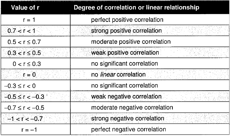
Correlation Coefficient:

‘r’

If the value of the correlation coefficient is positive, the direction of the relationship is positive

If the value of the correlation coefficient is negative, the direction of the relationship is negative

Measures how closely the relationship between two sets of data approximated to a linear relationship:

Lurking or Confounding Variable:

“No, although there is an observed association, we cannot assume that <explanatory variable> causes <response variable>.”

“There may be a casual relationship but it cannot be assumed it exists purely on the basis of there being an association.”

Linear Regression Residuals

The vertical differences between the obtained y values & the y values predicted by the linear regression line.

In sequences what does ‘term’ refer to:

Each number in the sequence is a term of the sequence.

E.g., in the sequence 4, 7, 10, 13, 16, 19, …

the first term is 4, the second term is 7, the third term is 10 & so on.

First Order Recurrence Relation:

Uses one existing term of a sequence to generate the next.

Tn + 1 = b x Tn + c , T1 = a

Second Order Recurrence Relation:

Uses the previous two terms of a sequence to generate the next

Recurrence Relation Recursive Rule:

Arithmetic:

An arithmetic sequence is a sequence of numbers such that the difference between any two successive members of the sequence is constant.

Tn+1 = Tn + d , T1=a

Common difference = d

*Term is Tn

*Term one term before Tn is Tn-1

*Term one term after Tn is Tn+1

*Term two terms after Tn is Tn+2

Recurrence Relation Recursive Rule:

Geometric:

Tn+1 = bx Tn + c , T1 = a

What happens to the terms of the sequence ‘in the long term’ i.e., as n → ∞

The sequence seems to be increasing/decreasing in approaching _____.

Explain why this ‘‘long term steady state situation’ occurs.

This steady state situation occurs because as n approaches infinity, the influence of the initial terms diminishes, and the behaviour of the sequence stabilizes around the increasing/decreasing <insert reciprocal b value i.e., a b value of 0.96 would be written as 4%> dictated by the recursive formula.

What is a Vertice:

A point where two edges meet

What is a Loop:

An edge that starts & ends at the same vertex

What Constitutes as a Multiple Edge:

If two or more edges connect the same two verticies.

What are directed edges/arcs:

Directed edges/arcs are indicated by an arrow.

What Constitutes a Simple Graph:

it must be unweighted & undirected with no loops or multiple edges.

What is a Walk:

A sequence of vertices in which there is an edge from each vertex to the next

What is a Closed Walk:

Any walk that starts or finishes at the same vertex is a closed walk.

What is an Open Walk:

Any walk that does not end at the starting vertex is an open walk.

What is a Path:

Path (in a graph)

A path in a graph is a walk in which all of the edges and all the vertices are different.

• No repeated vertices

• No repeated edges

What is an Open Path:

Open Path: A path that starts and finishes at different vertices.

What is an Closed Path/Cycle:

Cycle (Closed Path): A path that starts and finishes at the same vertex.

What is a Trail

A walk involving no repeated edges.

What is a Bridge:

An edge in a graph that if removed would leave the graph undirected.

What is a Complete Graph

Every vertices is connected to every other vertices by an edge.

What is a Planar Graph:

A graph that can be drawn without its edges crossing over.

What is Euler’s Rule:

v + f = e + 2

What is a Subgraph:

A graph showing a selection of vertices & edges from an original graph.

What is a Tree:

Any connected simple graph that contains no cycle

What are Bipartite Graphs:

A graph in which the vertices can be split into two groups such that every edge joins a vertex from one group to a vertex of the other group.

What is required for a network to be traversable:

Must be connected & have either zero odd vertices or exactly two odd vertices.

What is a Eulerian Trail:

A trail in a connected graph that travels every edge once & once only, repeated vertices are permitted.

What is a Eulerian Circuit:

A trail in a connected graph that travels every edge once & once only, repeated vertices are permitted that starts & finishes at the same vertex - therefore the graph is Eulerian if its traversable (starting & finishing at the same point)

What is a Semi-Eulerian Trail:

An open trail in a connected graph that travels every edge once & once only, repeated vertices are permitted

What is a Hamiltonian Path:

A path in a graph that visits every vertex in the graph once only with the possible exception of visiting the first vertex again at the end making the path a cycle.

What is a Hamiltonian Cycle:

A path in a graph that begins & ends with the same vertex & the closed path or cycle is said to be a Hamiltonian cycle.

What is required to be Semi-Hamiltonian:

A connected graph that contains an open Hamiltonian path, but not a Hamiltonian cycle is said to be semi-Hamiltonian.