AP Statistics

categorical variable

variable that cannot be quantified (e.g. M&M color, Skittle flavor)

quantitative variable

variable that can be expressed as a number

relative frequency

the number of times an event occurs divided by the total number of events occurring (e.g. the team won 70% (7/10) of their games)

marginal relative frequency

proportion of the whole (e.g. % of all students who chose music class)

joint relative frequency

combined proportions of the whole (e.g. % of all students who chose art as their favorite elective and math as their favorite core class)

conditional relative frequency

proportion of a part; this given that (e.g. % of the students who chose technology as their favorite elective given they chose math as their favorite core class)

segmented bar graph

bars are stacked to make up 100%

mosaic plot

segmented bar graph where width of the bars is proportional to the size of the group

association

when knowing the value of one variable helps us predict the other variable

discrete variable

variable with a countable number of values

continuous variable

variable with an infinite number of possible values

SOCS

Shape, Outliers, Center, Spread

unimodal

when a graph has only one peak

bimodal

when a graph has two peaks

non-resistant

measures of a distribution that are affected by outliers (mean, standard deviation)

IQR (interquartile range)

represents the middle 50% of a dataset, spanning from the 25th to 75th percentile

interpretation of standard deviation

“The context typically varies by standard deviation from the mean of .

1.5IQR method for outliers

low outlier < Q1 - 1.5IQR

high outlier > Q3 + 1.5IQR

2SD method for outliers

low outlier < mean - 2SD

high outlier > mean + 2SD

five-number summary

minimum, Q1, median, Q3, maximum

examples of comparative language

greater than, less than, similar to

adverbs for describing a distribution

strongly, roughly, approximately, moderately

percentile

The Pth percentile is the value that has P% of the data less than or equal to it

z-score

number of standard deviations a value is from the mean; shows position relative to other values in the distribution

interpretation for z-score

“Context is z-score standard deviations above/below the mean of .”

linear transformation of data

add/subtract: only mean changes

multiply/divide: both mean and SD change

standardizing a distribution

mean = 0, SD = 1, shape is the same

empirical rule

68% of the data is contained within 1 SD of the mean, 95% is contained within 2, and 99.7% is contained within 3

DUFS

Direction, Unusual features, Form, Strength

unusual features

outliers or clusters

form

linear or nonlinear

strength

how close the data is to the form

r for correlation

direction: +/-

form: linear

strength: between -1 and 1

interpretation for r

“The linear relationship between x and y is strength and direction.”

interpretation for r² (coefficient of determination)

“r²% of the variation in y i accounted for by the linear relationship with x.”

extrapolation

the process of estimating unknown values by extending or projecting from known values

residual

actual-predicted

interpretation for residual

“The actual context was residual above/below the predicted value for x = #.”

interpretation for y-intercept

“When x = 0 in context, the predicted y context is y-intercept.”

interpretation for slope

“For each additional x context, the predicted y context increases/decreases by slope.”

least squares regression line (LSRL)

minimizes the sum of the residuals

residual plot

If there is no clear pattern in the residuals, it is appropriate to use a linear model

interpretation for standard deviation of the residuals (s)

“The actual y context is typically about s away from the number predicted by the LSRL.”

interpretation for r² of LSRL

“About r²% of the variability in y context is accounted for by the LSRL.”

LSRL outliers

points with high residuals

LSRL formula

ŷ = a + bx

LSRL slope formula

b = r(Sy/Sx)

LSRL constant formula

a = ȳ - bx̄

convenience sample

participants are chosen based on access and availability; non-random

stratified random sample

splits population into homogeneous groups based on shared characteristics (Taylor Swift concert rows)

cluster sample

split population into heterogeneous groups, select a number of groups, and sample everyone in each group

systematic random sample

choose random starting point, select participants at equal intervals (e.g. every 5th person)

standards for good sampling methods

low bias, low variability

undercoverage

some people are less likely to be chosen (e.g. people without cell phones)

non-response

people can’t be reached or refuse to answer

response bias

problems in data gathering instrument/process (question wording, people don’t tell the truth, etc.)

experiment

procedure where treatment is imposed on experimental units

observational study

no treatment is imposed on participants

experimental units

who/what the treatment is imposed on

criteria for a well-design experiment

comparison of 2+ treatments, random assignment, replication (more than one subject in each treatment group), control

benefit of random assignment

shows causation

benefit of random sampling

results can be generalized to the population

matched pairs design

subjects are paired based on similarity and then randomly assigned to a treatment (e.g. similar SAT scores) OR each subject receives both treatments (e.g. two sides of a leaf)

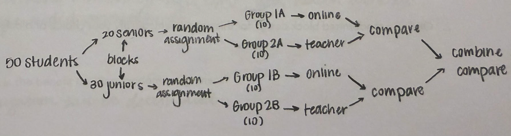
randomized block design

subjects are separated into blocks based on similarities and randomly assigned treatments within each block (e.g. testing student performance in different grades)

statistical significance

when results of an experiment are unlikely (<5%) to have occurred by chance

law of large numbers

simulated probabilities tend to get closer to the true probability as the number of trials increases

long run relative frequency

more predictable than short run relative frequency

complement rule

probability of an event NOT occurring; P(A^c) = 1 - P(A)

addition rule

P(A∪B) = P(A) + P(B) - P(A∩B)

*if events A and B are mutually exclusive, they cannot occur together and P(A∩B) = 0

mutually exclusive

when events cannot occur at the same time (e.g. heads and tails)

independent

the outcome of one event does not affect the outcome of the other

superscript c

denotes a complement; the probability or trials where something does not happen

when combining random variables…

add/subtract means, add variances

binomial distribution

a distribution with a fixed number of trials and two possible outcomes

formula for binomial probability

p_x = (nCx)p^xq^n-x

n = number of trials

x = number of successes

p = probability of success

q = probability of failure

BINS

Binary (success or failure), Independent trials, Number of trials is fixed, Same probability of success (p)

calculator function for P(x = r)

binompdf(n, p, x)

calculator function for P(x ≤ r)

binomcdf(n, p, x)

calculator function for P(x ≥ r)

1 - binomcdf (n, p, n-x)

mean for binomial distribution

µ = np

standard deviation for binomial distibution

σ = √np(1-p)

interpretation for mean of binomial distribution

“After many groups of n trials, the average number of successes is µ.”

interpretation for the standard deviation of binomial distribution

“The number of successes typically varies by σ from the mean of µ.”

large counts condition

np ≥ 10 and n(1-p) ≥ 10; allows for the use of a normal distribution and its calculations

10% condition

n ≤ .10N; allows for sampling without replacement

BITS

Binary (success or failure), Independent trials, Trials until success, Same probability of success

formula for geometric probability

p(x = k) = (1-p)^k-1p

p = probability of success

k = number of trials

shape of geometric distribution

skewed right

shape of chi-squared distribution

skewed right

shape of t distribution

normal with greater area in the tails

mean of geometric distribution

µ = 1/p

standard deviation of geometric distribution

σ = √(1-p)/p

sampling distribution

distribution of values of a statistic for all possible samples of a given size from a given population

as n increases…

variability decreases

biased estimator

consistently over/underestimates the true population parameter

unbiased estimator

results in a sample mean that is equal to the population mean

mean of sampling distribution for p̂

µ_p̂ = p

standard deviation of sampling distribution for p̂

σ_p̂ = √p(1-p)/n

mean of sampling distribution for x̄

µ_x̄ = µ