Qualifying Exam: Signals and Systems

Analog signal

amplitude (y axis) can take on infinite number of values

Continuous time signal

independent variable (x axis) can take on an infinite number of values

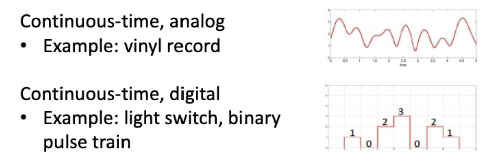
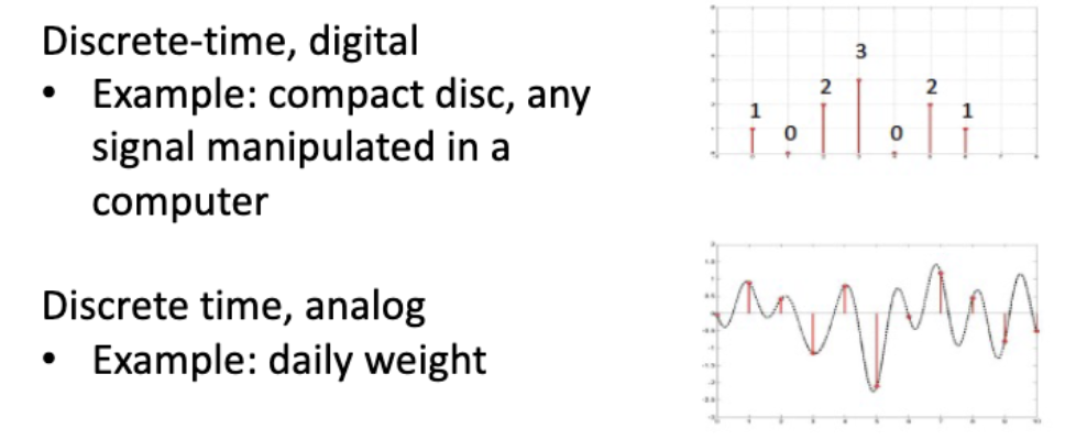
Digital signal

amplitude (y aics) can take on finite number of values

Discrete time signal

independent variable (x axis) can take on an finite number of values

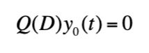
Zero input response

what the system does with no input at all (due to initial conditions like energy store in capacitors)

ytotal (t) = yzs (t) + yzi (t)

Zero state response

output of the system with all initial conditions at zero; found using the convolution integral

ytotal (t) = yzs (t) + yzi (t)

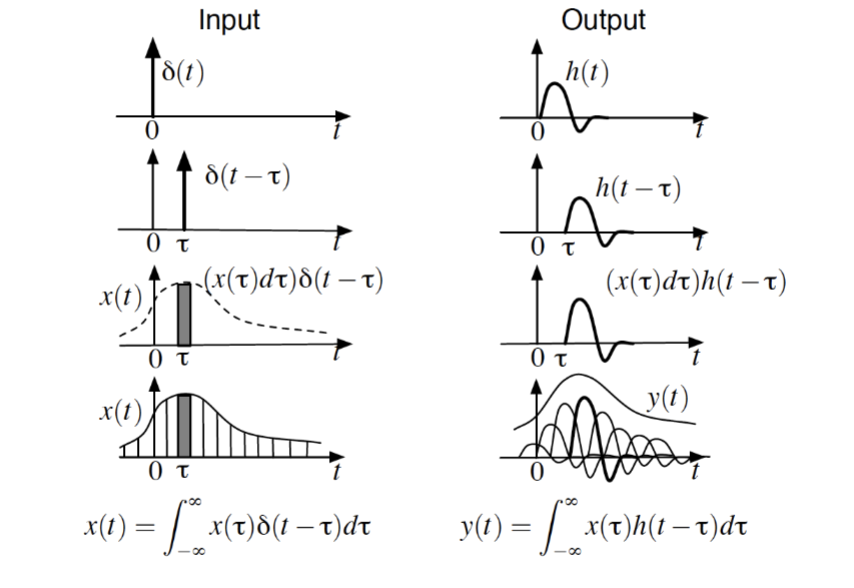
Impulse response

the output of the system at a time (t) to an impulse at time (𝜏)

h𝜏 = H(δ𝜏)

Unit impulse response

h(t)

Response of the system to a unit impulse input

Characteristic of the system, and used for finding the zero-state response

Convolution

Convolution combines an two signals: an input signal x(t) and the system’s impulse response h(t), to produce a third signal y(t)

y(t) = x(t) * h(t)

This can be used to find either the zero-state response x(t) or the unit impulse response h(t)

Zero-state stability: BIBO

BIBO Stable: application of a small input produces a response that eventually decays to zero

BIBO unstable: application of a small input produces an unbounded (ever increasing) response

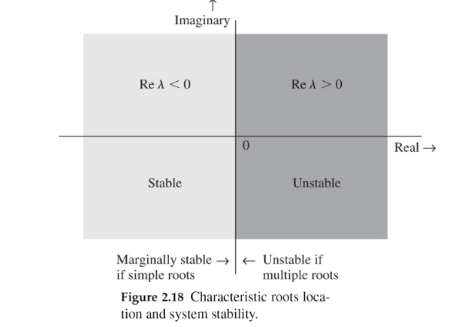
Zero-input stability: Internal (Asymptotic)

Internally stable: application of nonzero initial conditions produces a response that eventually decays to zero

Internally unstable: application of nonzero initial conditions produces a response that increases with time

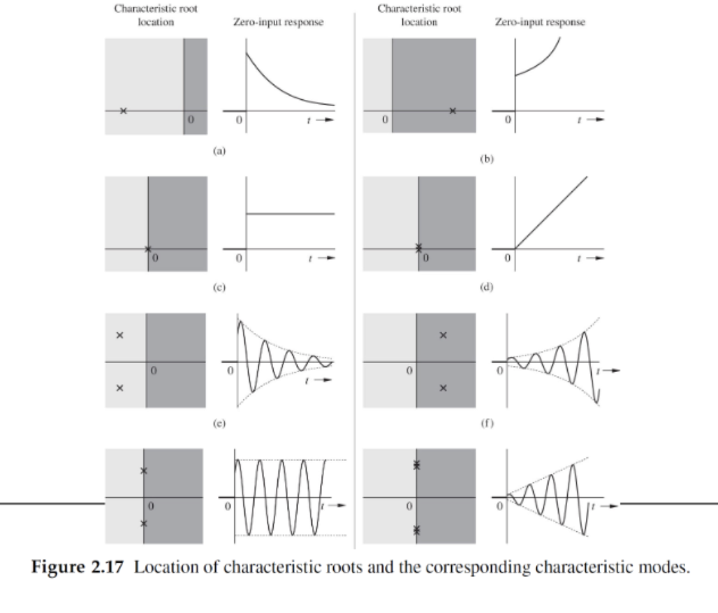
Can be determined using characteristic modes

Fundamental frequency of sines and cosines (𝜔₀)

Fundamental frequency is the greatest common factor of all the frequencies in the series

A signal composed of sines and cosines of frequency 𝜔₀ and all of its harmonics is a periodic signal with the same period as that of the fundamental, regardless of the values of the amplitudes of each sine and cosine.

Trig series of a periodic signal

Finding the Fourier series for a periodic signal can be used to determine contributions of each of the periodic signals present in the signal

Helps determine frequency spectrum

Fourier series

a method of representing a periodic signal as a weighted sum of sinusoids, or everlasting exponentials whose frequencies lie along the j𝜔 axis in the s plane

Every periodic signal has a time domain and frequency domain representation

Fourier series: time vs frequency domain

time domain shows how a signal’s amplitude changes over time

frequency domain shows how much signal lies within frequency bands

Fourier transform translates between the two, decomposing signals into the sums of sinusoids

Bandwidth

the difference between the highest and lowest frequencies of the spectral components of a signal

Fourier transform

Transforms from time domain to fourier (frequency) domain

Amplitude and phases together make up the frequency spectra of x(t), constituting the frequency-domain description of x(t)

Fourier transform: constant

a constant signal in time corresponds to an impulse at zero frequency

Fourier transform: Sines

Fourier transform of sin/cos at a frequency f₀ only has energy exactly at ± f₀

One positive direction, one negative direction

Fourier transform: Cosines

Fourier transform of sin/cos at a frequency f₀ only has energy exactly at ± f₀

Both positive direction

Scaling property: Bandwidth effect

Doubling the signal duration halves its bandwidth, and vice versa

The bandwidth is inversely proportional to the signal duration or width

Convolution and Convolution Theorem

convolution in the time domain is multiplication in the frequency domain

Conv. Theorem: Given two signals x1(t) and x2(t) with Fourier transforms X1(f) and X2(f),

(x₁*x₂)(t)<=>X₁(f)X₂(f)

Modulation (Frequency Shifting Property)

Modulating a signal by an exponential shifts the spectrum in the frequency domain.

Modulation by a cosine causes replicas of X(f) to be placed at plus and minus the carrier frequency; replicas are called sidebands

Modulation vs Demodulation

Modulation varies a high-frequency carrier signal with low-frequeny information signal

Demodulation is the reverse process, and extracts the original information signal from the carrier at the receiver

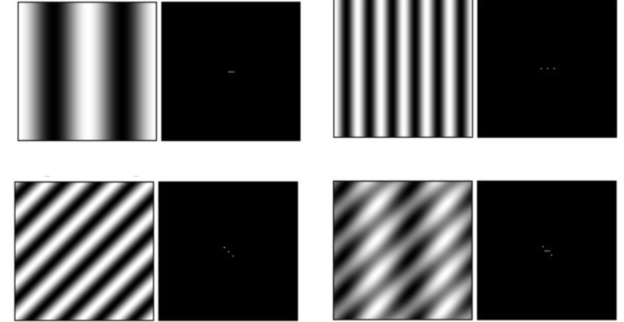
2D Fourier transform

The Fourier transform of a sinusoidal function presents as a Fourier series, with the central dot indicating the a₀ or dc components and the dots on either side indicating the frequency component. For higher spatial frequency images, the dots are offset further away from the dc component

Natural (Homogeneous) and Forced (Particular) Responses

Homogeneous response: represents transient response of the system when the input is zero

Particular response: represents a forced steady-state response driven by a particular input

Fourier series vs Fourier transform

Fourier series: for discrete index, calculated using summation

Fourier transform: for continuous index, caculated using integral

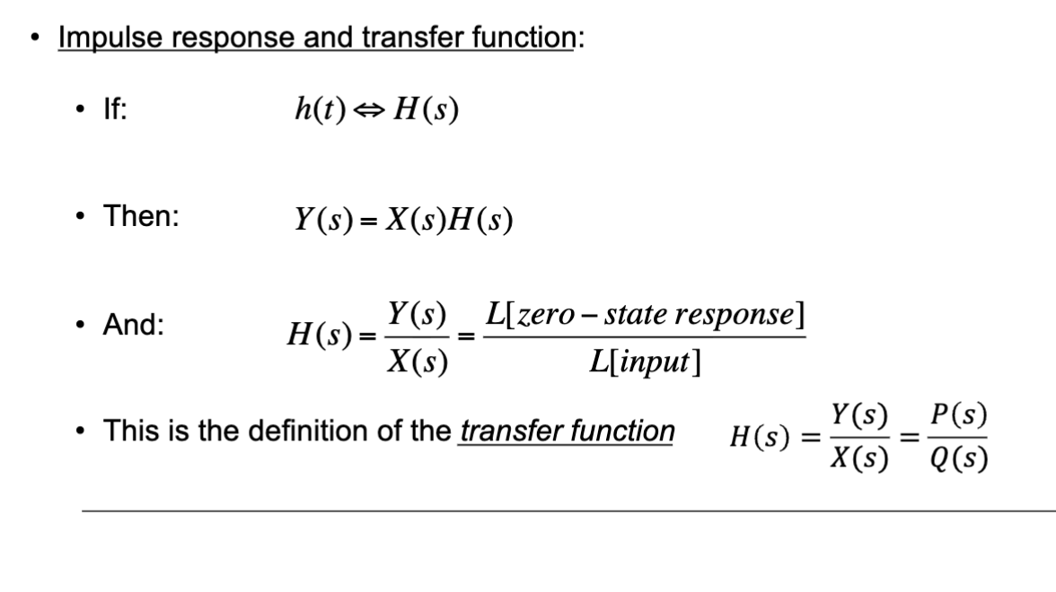
Impulse response and transfer function

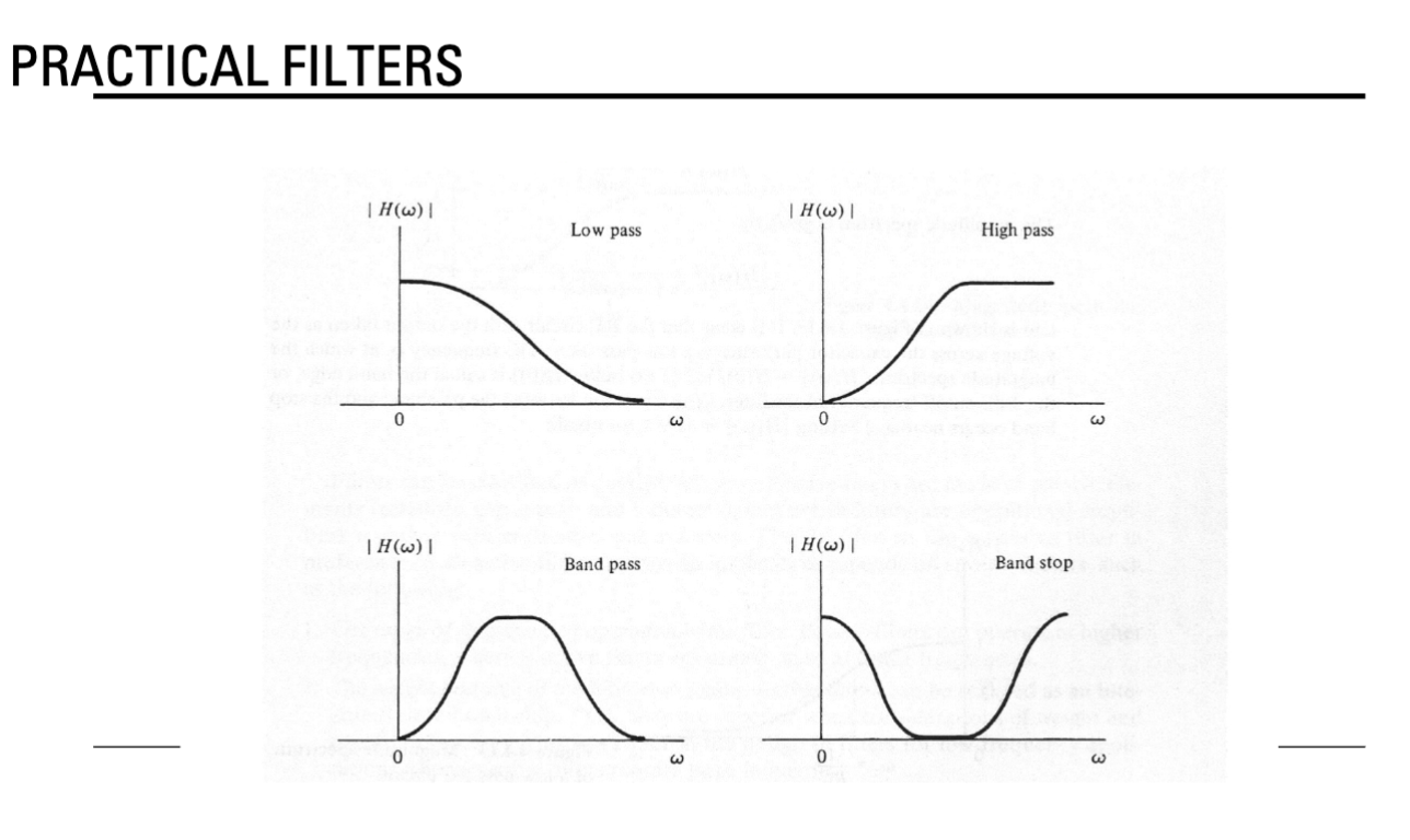
Filtering

the process by which the essential and useful part of a signal is separated from the undesirable components (noise, for example)

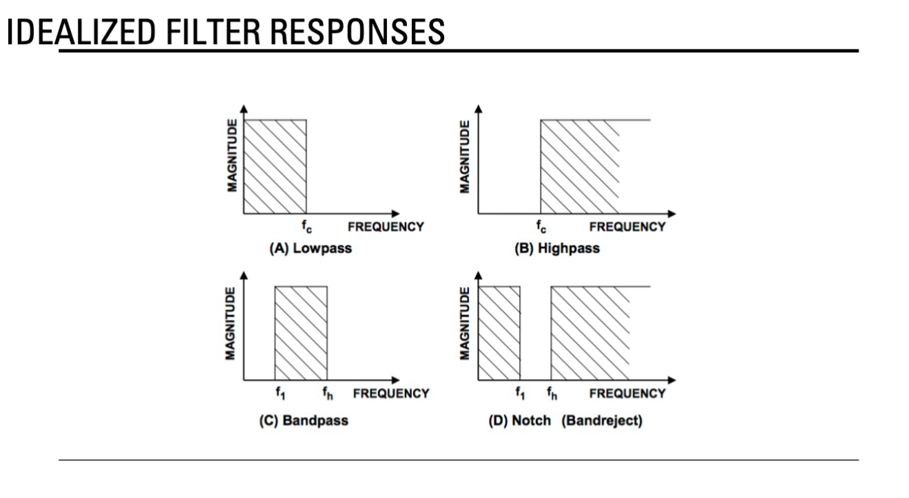
Idealized filters are impractical

Idealized filters are impractical because the impulse response of the filter in the time domain requires infinite time to remove the unwanted frequency components, and is anticausal

Fourier transform in image processing

Filter is applied in the Fourier domain, as it can be done using multiplication in Fourier domain rather than convolution in the space domain

Then, the inverse Fourier transform is used to obtain the filtered image

Nyquist Sampling Theorem

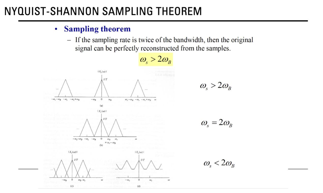
Effects of under/over sampling: aliasing

Aliasing occurs by undersampling

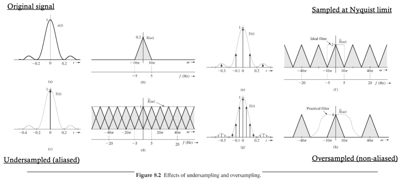
Overcoming aliasing

Sample at the Nyquist rate or greater

If sampling fast enough is not possible, then apply a low-pass filter to the input signal such that the sampling rate satisfies Nyquist for the filtered signal

Best to do both- can’t measure higher frequencies than ½ of sampling frequency accurately due to aliasing

Laplace Transform

Much like Fourier transform, converts time-domain signals into the frequency domain

LaPlace may be used to solve for transient analysis with unstable (exponentially growing) signals that cannot be accommodated by the Fourier transform

Relevance of Fourier transform in SIM imaging

• Fourier analysis of raw data generated by the microscope in the rear focal plane of the objective

• Deconstruction of observed fluorescence frequencies into their components, including the spatial frequency of the sinusoidal illumination structure, whose Fourier transform has three components

• High frequency information may undergo frequency mixing with the illumination structure and be displaced into the observable region as moiré fringes