Principles of Microeconomics - Semester 2 key terms

Conditions for Price discrimination:

1. Sellers must be price makers

   1. Must be able to influence market price / price-setting power

2. Buyers must be different and sellers must be able to identify

   1. Market differentiation / distinguish consumers

3. Consumers must NOT be able to participate in arbitrage

   1. Cannot - buy at low and sell to buyer who would have paid a high price

Characteristics of market structure:

Market structure: A structure that refers to characteristics of a market that may affect trades

Characteristics:

• n. and size of sellers (firms)

• Barriers to entry

• Product differentiation

• n. and size of buyers (individuals)

  • Assumption market = product market

Perfect competition:

• Extreme on the competition spectrum, with unrealistic assumptions with few IRL examples

• However, agricultural and financial markets are close.

Rules of perfect competition:

Rule 1: Marginal output rule	Rule 2: Shutdown
MR = MC, prevent shut down	Shutdown if p < AC
MR > MC, then P increases (^ = TR - TC)	SR: p < AVC 😟
	LR: p < LRAC 😟

Assumptions of Perfect competition

• Buyers = Price Takers

• Complete information

• Sellers = Price Takers

• All firms have no market power

• Free entry (L-R decision)

  • capital —> employ —> Q rises

Characteristics of perfect competition:

• Many small sellers

• Low B2E

• Undifferentiated products

• as output is a small fraction of total industry output

• Firms do not actually compete with each other e.g. Essex and Somerset farmers

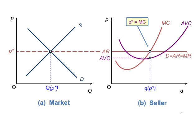
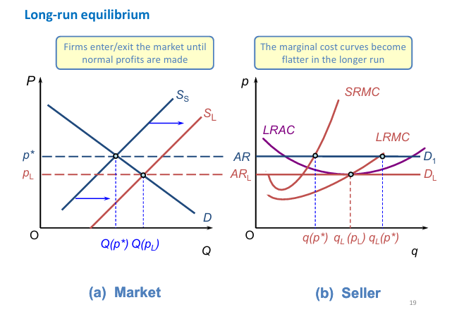
LR EQ of Perfect competition:

• Occurs when firms earn zero profit at the break-even price

• Change due to factor variability and low barriers to entry

• Sellers and buyers produce or purchase as much as the other desires

  • TF, sellers make NP in the LR

• Third condition - Incumbent sellers stay and potential sellers do not enter

• No incentive to enter or leave the industry as they break even and can invest elsewhere

Assumptions of a Monopoly:

• Buyers are PT and complete information

• Monopolist = Price maker with price setting power

  • Seller sells more with lower price

  • Seller’s output choice does not trigger a reaction from competitors

• Entry is BLOCKED; legal, structural or strategic B2E

Monopoly market structure:

• One large firm

• High B2E and differentiated products

• Opposite of PC which include many small firms, low B2E and undifferentiated product

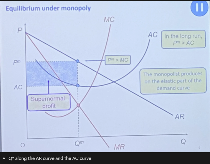
Monopoly EQ

• Q* along the AR curve and the AC curve

• Pm = monopolist price

• SNP at Qm, MC through minimum of AC

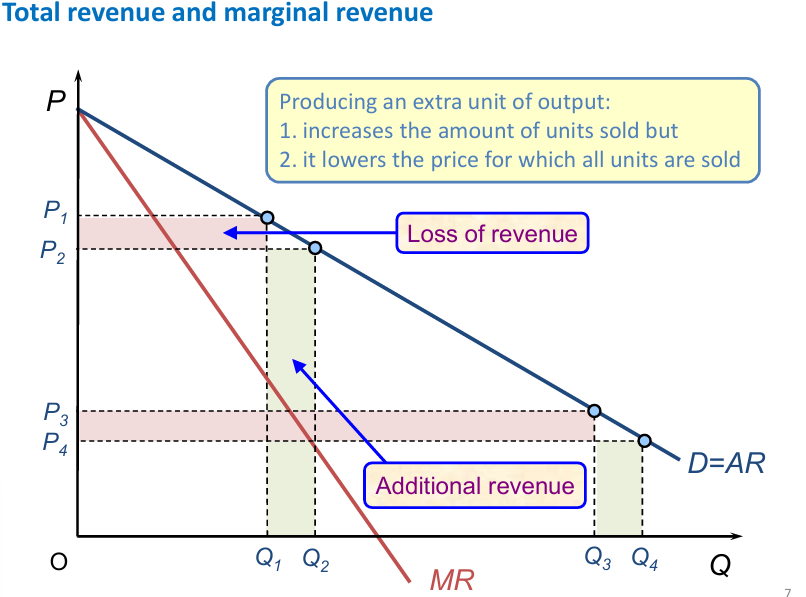
• Produces on the elastic part of the demand curve

Positive MR —> TR rises with extra Q unit, elasticity > 1

Negative MR —> TR falls with extra Q unit, 0 < e < 1

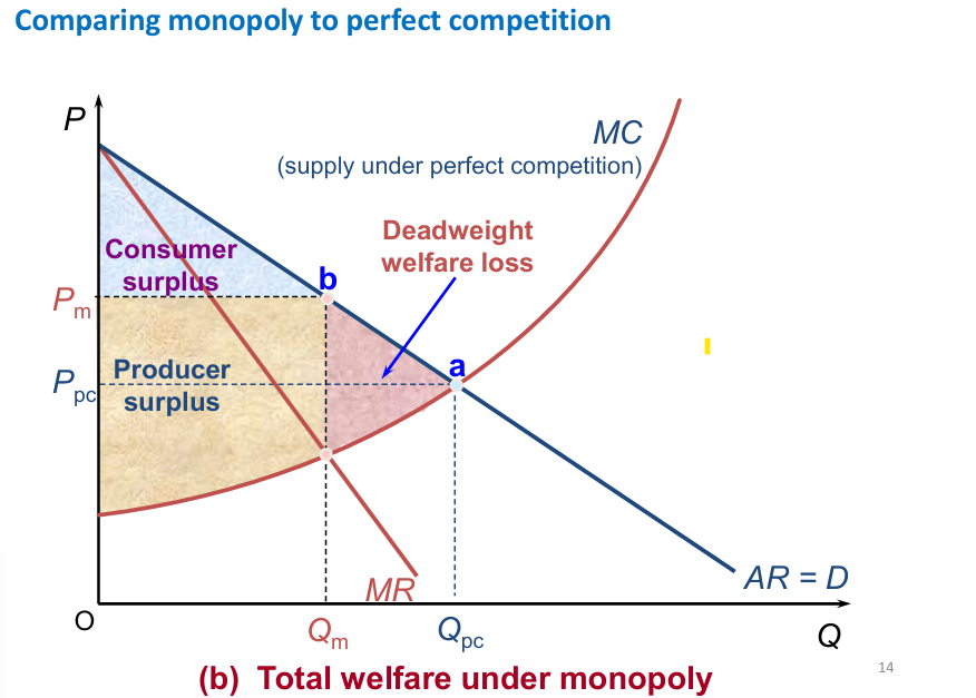
Monopoly vs perfect competition:

Monopoly is worse in terms of total welfare (PS + CS) than PC on the consumer

Consumer surplus: different between demand curve and the price (above P*)

Producer surplus: difference between price and supply curve (below P*)

• Producer surplus has increased (compared to usual CS PS diagram),

• Consumer surplus has decreased

• DWL has arisen

• Lower quantity and higher price

• Total welfare has fallen compared to under PC

Monopoly inefficiency:

Monopolies are allocatively inefficient as consumer surplus is lower than perfect competition and there is no incentive to reduce price

• This creates DWL

• The firm does not maximise producer and consumer surpluses

First-degree price discrimination:

• Sellers charge each buyer the max price the buyer is willing to pay

• Another unit is sold at a lower price so TR increases but there is no marginal forthcoming decline of price level due to PD. MR = AR

  • TR = p = AR

e.g. Miss Rich is willing to pay £40 for the first unit and £20 for the second unit

• would be charged both these prices for both these units

• Unlikely in the real world, but an important foundation

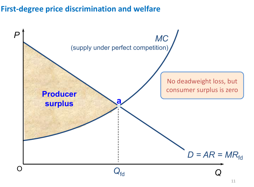
First-degree price discrimination and welfare diagram:

• Produces at the same point of Perfect Competition

• NO DWL or CS; this is because every consumer is charged at their max willingness to pay and thus reap no additional benefit

• Monopolist changes different prices for each unit sold

• Produces more than what it would if it couldn’t price discriminate

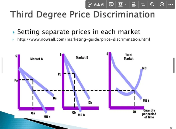
Third-degree price discrimination:

• seller can identify groups of buyers and differ prices charged

  • Grouped by characteristics e.g. students / non-students

  • Grouped by location e.g. HIC vs LIC

• Marginal costs increase in output

• Must be able to identify markets, keep them separate and maintain different prices, whilst also preventing arbitrage

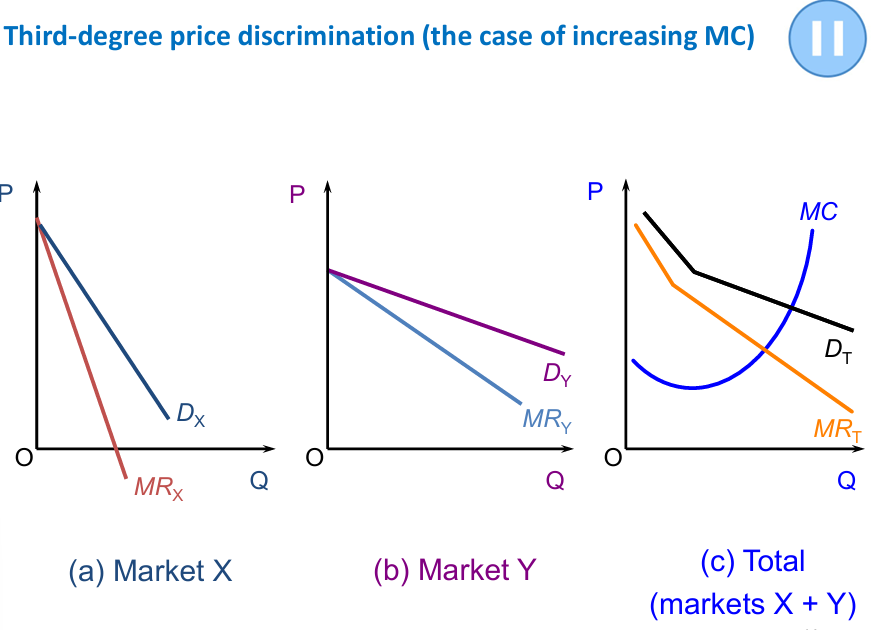
Third-degree price discrimination diagram:

• Market X and Market Y differ depending on level of demand

• Summing MRx and MRy gives the total market MR curve

  • intersecting with MC —> Pmax and draw line across, then connect to x axis

• Market X - charged higher price with more inelastic demand

• Market Y - charged lower price with more elastic demand

• Total = Market X + Market Y

• CS = positive, higher than first degree

• DWL where prices > MC

• price lies between two groups

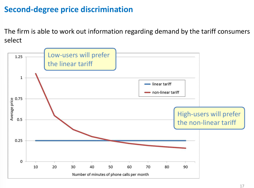
Second-degree price discrimination and linear / non-linear tariffs

A seller can use a menu of “non-linear tariffs” to get buyers to reveal preferences when they select their preferred tariff

Linear tariff: same price charged for every unit sold

• 25p per minute for phone calls

Non-linear tariff: average price per unit changes

• £10 per month and 5p per minute

Characteristics of Monopolistic Competition:

• many sellers in competition

• price-setting power

  • Seller can raise price and not lose all its sales

• low barriers to entry

• differentiated products / imperfect substitutes

  • horizontal: same quality, diff tastes

  • vertical: quality differs, same tastes

Assumptions of Monopolistic Competition

• buyers are price takers

• complete information

• Sellers are price makers

  • Sells more with lower price

  • Does not trigger a rival reaction if Q changes

• Free entry - LR entry has no incurring costs; LR decision (FoP)

Pub example of symmetric sellers in Monopolistic competition:

Symmetric demand:

• 4000 people who go to 40 pubs

• at market price, each pub would have 100 people

+10 pubs with constant pubs

• Each pub would have 80 regulars (4000 / 50 pubs)

• Incumbent lose 20 people to entrants

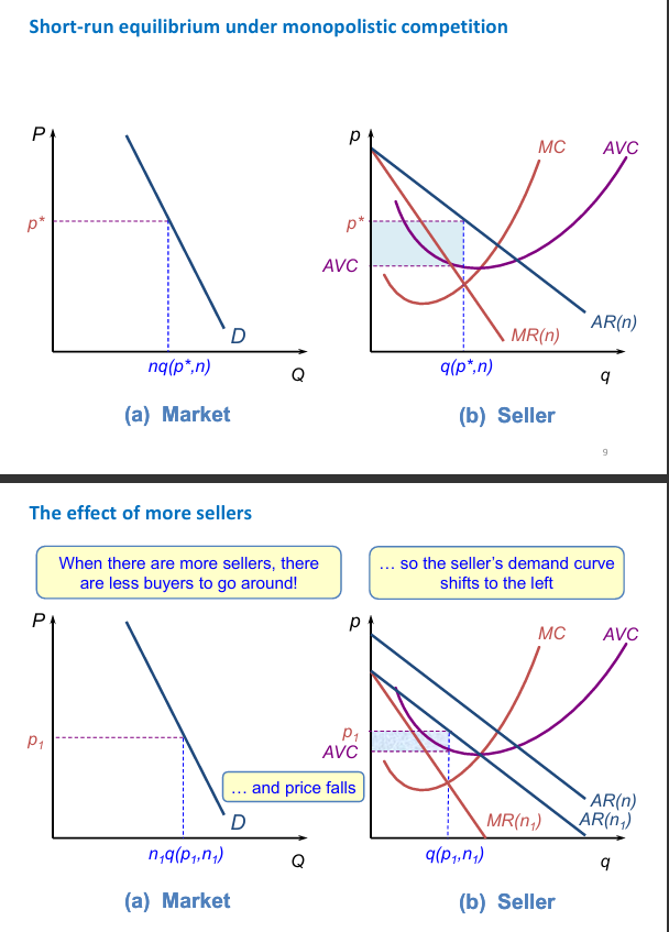
Short-run Equilibrium for Monopolistic Competition

• R EQ is just price maker

• AVC on y axis is correlating to Q*

• demand is down-sloping in the market with EQ

• more sellers —> less buyers so EQ price falls, thus shifting along demand curve

• demand curve shifts to the left (ARn1)

• MR curve shifts to the left (MRn1)

• New Q (p1n1) and price (p1)

• This means price falls and AVC rises

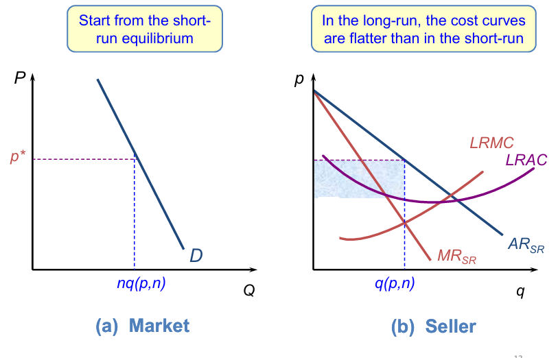
Long-run equilibrium of Monopolistic Competition:

• All factors variable and other sellers can freely enter

• Sellers make Normal profit in the LR

• In the LR, cost curves are flatter

• Firm is more efficient as costs fall

• firms will enter the market until LR profit is zero

  • P (LR) = AR (LR) = LRAC

• LR price = Where MR and MC in the LR intersect to meet the AR curve

• Zero economic profit

PC vs MC vs Monop:

Feature	Perfect Competition	Monopolistic Competition	Monopoly
1. Output rule	MR = MC	MR = MC	MR = MC
2. Short-run profits?	Supernormal	Supernormal	Supernormal
3. Price taker?	Yes	No	No
4. Price	Equals MC	Above MC	Above MC
5. Efficient output?	Yes	No	No
6. Number of firms	Many	Many	One
7. Entry in long run?	Yes	Yes	No
8. Long-run profits?	Normal	Normal	Supernormal

Dominant strategy:

The strategy that provides a player with the highest payoffs, regardless of an opponent’s strategy

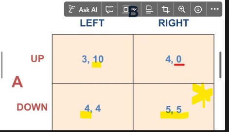
Nash Equilibrium:

There is no dominant strategy equilibrium

• When no player can do better than their chosen strategy, given their beliefs of how the other players will play

1. Best response against opponent conjecture

2. Conjectures must be correct

Nash here is 5,5 (double underline)

Subgame perfect nash equilibria:

Subgame perfection is a refinement on the Nash equilibrium that allows us to make better predictions for sequential move games It requires there to be a Nash equilibrium in every “subgame”

Subgame perfect nash equilibria example:

1. A + UP —> B + Right (16,12)

2. A + Down —> B + Left (14,14)

3. A would go up

4. Nash Equilibrium is Up, Right

Correct conjectures

Assumptions of Oligopoly:

• A1 Buyers are price takers + A2 complete information

• A3 Sellers = Price makers ; downward sloping demand curve, as well as output choices triggering a reaction from its rivals

• A4 Entry is BLOCKED; SR and LR

Cournot’s model of Oligopoly (specific assumptions):

• A1 two sellers (duo-polists)

  • they choose the level of output to produce and make simultaneous decisions

• A2 further entry is blocked to sustain the number of firms

• A3 Homogenous products (for simplicity)

• A4 the market’s inverse demand = P = a - Q

  • P = market’s inverse price

  • a = intercept of the inverse D curve

  • Q = total amount of output in the market

  • a > 0

  • e.g. if Firm A produces Qa + B produces Qb then Q = Qa + Qb

    • P = a - Qa - Qb

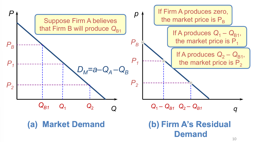
Firm A residual demand curve in Cournot’s Oligopoly Model:

• the RDC = Firm’s demand curve, given the rival output (market demand that its rival has not supplied)

• Firm A believes Firm B will produce QB1

  • A output = zero —> MP = Pb

  • A output = Q1-Qb1 —> MP = P1 (what is left by B is produced)

  • A output = Q2 - Qb1 —> MP = P2 (what is left by B is produced)

  • Match each point on Firm A’s diagram and connect to create the residual demand curve

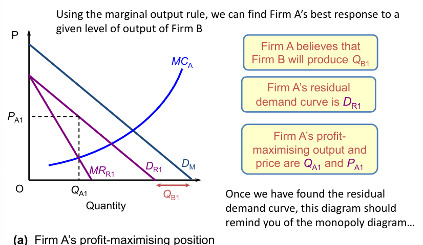
How to find Firm A’s best response, given Firm B’s output —> Pmax under Cournot’s Nash Equilibrium:

• Assume B will produce Qb1 —> shift-in by QB1 (MD - rival output) —> DR1

  • Find MRr1 curve as usual

  • Cross over with MC for A ; MCa

  • price = PA1

1. Firm A believes what output B will produce

2. Establish residual curve

3. Shift curve by rival output

4. Determine P-max

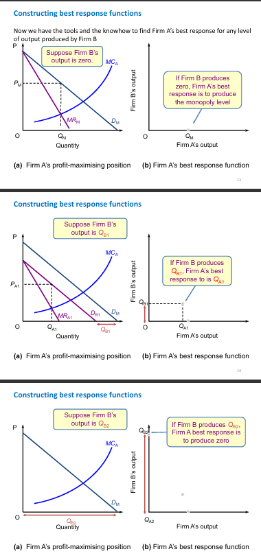
Constructing best response functions:

1:

1. Firm B output = zero, so there is no rival output

   1. Best response = to produce at monopoly level

   2. Qm (on output axis)

2:

1. Firm B output = QB1, so subtract QB1 from market demand Dm to find what’s left

   1. best response = produce at Qa1, where MCa meets MRa1 (profit max)

   2. Qa1 on output axis

3:

1. Firm B produces Qb2, complete rival output

   1. best response = produce zero at Qa2

   2. Qa2 on y-axis (where output is zero and price is high); same point where Dm meets y-axis

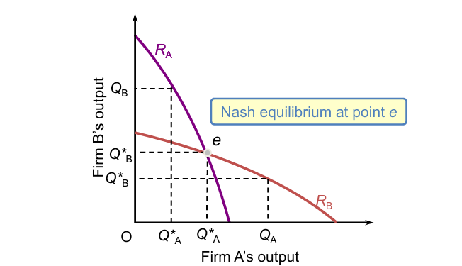
Cournot’s Nash Equilibrium diagram:

Nash equilibrium consists of two output levels,

1. Given that Firm B produces Q*b, Firm’s A profit is maximised by producing Qa

2. Given that Firm A produces Q*a, Firm B’s profit is maximised by producing Qb

• To solve for the Nash equilibrium, we must find the firms’ best responses!

• Ra = Firm A’s best response —> Pmax

• Rb = Firm B’s best response —> Pmax

• A duopolist’s output level is determined by the marginal output rule

We need to find each duopolist’s MR curve from their D curve

Comparisons of Cournot Oligopoly to Monopoly and Perfect Competition

• Perfect competition, MCA and MRM

• Monopoly still has higher price

Bertrand’s model of Oligopoly Assumptions:

1. two firms, duopolists, simultaneous price-setters

2. entry is blocked

3. Firms have the same constant MC, c, and no fixed costs

   1. increasing MC is upward curve, whilst constant is where MC = AC

4. Homogenous products, not differentiated

   1. buyers purchase cheaper good

5. Market demand is: Q = a - P

   1. Q = TD when lowest price is P, where a > 0

   2. If Firm A sets Pa below Firm B’s price of Pb, Q = a - Pa If Firm A sets Pa above Firm B’s price of Pb, Q = a - Pb

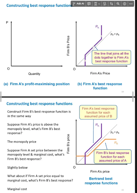
How to construct Bertrand best response function:

1. Set first point where P1 = Q1 as Firm A believes Firm B will set the same price

2. Find the residual demand curve which is DR, according to Firm A’s demand

3. Find points of Pmax which are Qa1 and Pa1, where MR crosses MC and complete

4. To create best response function, draw corresponding price diagram using 45 degree line (as both are simultaneous) and correlate Pm (from step 2) and the believed B price at b1

5. New scenario - Firm B price is below, same thing correlate Pb2

6. Correlate dots on Firm A best response function

7. Draw the inverse for Firm B on the best response function diagram

Thus this is the Bertrand-Nash EQ; where the two firm’s best responses intersect

Comparing Bertrand Nash EQ with Monopoly and PC in terms of price and welfare:

• Duopolists set a lower price than the monopoly

• Duopolists set the same price as the MP of PC and there is no DWL, maximised welfare

Bertrand Paradox and its 4 solutions:

Bertrand Paradox

• Suppose there is one firm (monopolist) —> high P

• One firm enters and sells identically, setting price under PC

• We go from Extreme of Monopoly —> Extreme of PC???

Solutions:

• Product differentiation

  • sellers don’t lose all of their customers when prices are higher

• Capacity constraints

  • controls residual demand if control supply

• Incomplete information

  • lower prices cannot attract if those are unaware

• Repeated interaction

  • less intense competition

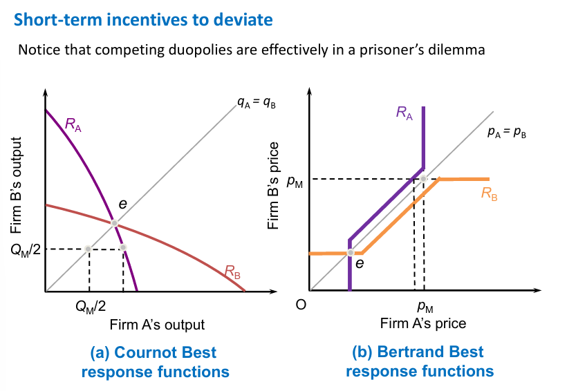
Bertrand and Cournot Pure Strategy Nash Equilibrium, and similarity to the Prisoner’s Dilemma:

• Betrand - Pure Strategy Nash Equilibrium:

  • Equilibrium E where Firm A price = Firm B price

  • Collusion:

    • Both firms could collude and set higher prices where Pm= PM

    • This goes from HB VA —> VB HZ

      • Incentive to deviate

        • e.g. firm could increase onto its best response function —> Pmax (purple) and vice versa

• Cournot - Pure Strategy Nash Equilibrium

  • Equilibrium E where Firm A price = Firm B price

  • Collusion:

    • both firms could restrict output (half) where Qm/2 = Qm/2, they share Monopoly profits and both are in equal positions

      • Incentive to deviate

        • e.g. firm could pr

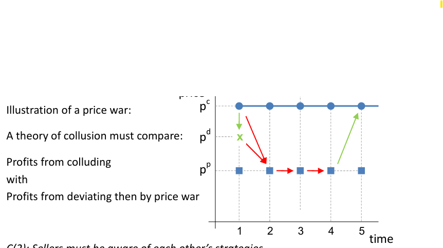
Conditions necessary for Oligopolists to collude:

1. Sellers must interact repeatedly

   1. Incentive to deviate must be counteracted by a credible L-T punishment, usually a price war (period of low prices)

2. Sellers must have complete information of each other’s strategies

   • if they are not aware, then a price war cannot be threatened

Infinite Prisoner’s Dilemma:

• The one-shot Nash Equilibrium (if played ONCE), is (deviate, deviate)

  • Both earn (75.75)

• Cooperation —> 150,150 to benefit, but both would have an incentive to deviate to earn 200 instead of 150, at the expense of the other firm .

  • Is (cooperate, cooperate) a Nash Equilibrium of the repeated game?

Grim trigger strategy in collusion:

• Each firm will cooperate, as long as the other has always done so

• If a player deviates, both firms revert to playing the one-shot Nash equilibrium (deviate, deviate)

• Punishment - price war forevermore.

Calculating present value of future payoffs:

Having £100 today =! £100 in the future:

• in one period the future, assume r = 0.05 (IR), so £100 —> £105

Having £100 in one period’s time equivalent to today:

If £X is invested

X + (X x 0.05) = X (1 + 0.05) or X x 105%

X (1 + 0.05) = 100

X = 1 / 1.05 (100) = 95.24

£100 tomorrow is equal to δ(100) today where δ = 1 / (1+r)

Having £100 in two period’s time equivalent to today:

If £X is invested

X (1+0.05)^2 = 100

X = 1 / (1.05)^2 x 100 = 90.71

£100 day after tmrw = δ^2 (100) today, where δ = 1 / 1+r

Formula here: X = (1 / (1+r)^t )) x 100 = δ^t x 100

X = (1 / (1+r)^t )) x 100 = δ^t x 100

Expected presented discounted value of this stream of payoff =

X (δ + δ^2 + δ^n + …..) =~ X δ / (1-δ)

period 1 = X x δ = Xδ

period 2 = X x δ^2 = Xδ^2

period n = X x … = Xδ^n

Expected present discounted value of this stream of payoff =

X (δ + δ^2 + δ^n + …..) =~ X δ / (1-δ)

If you sub δ = 1 / (1+r), then Xδ / (1-δ) = X /r

Factors of production, units and cost to firm:

• Labour: people available for employment —> output

  • Units: n. people, work hours

  • cost to firm: wage, salary

  • Variable in SR

    • LR - capital can replace it

• Capital: machines and equipment used by labour to produce output

  • units: n. machines, tools, factories

  • cost to firm: rent, price

• Land: site of production

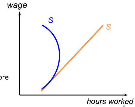
Supply of labour by an individual:

Two main costs: sacrificing leisure and unappealing work / high disutility

Substitution effect:

• Higher wages —> more hours worked; greater OPPC of leisure

Income effect:

• Higher wages —> afford more leisure time

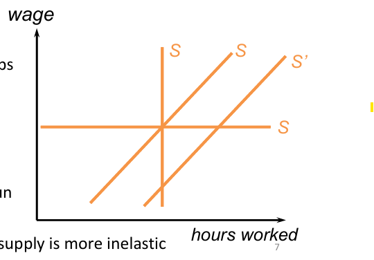
Supply of labour (to an employer and the market):

• Employer wage taker —> perfectly elastic supply curve

• Employer wage maker —> upward sloping supply curve

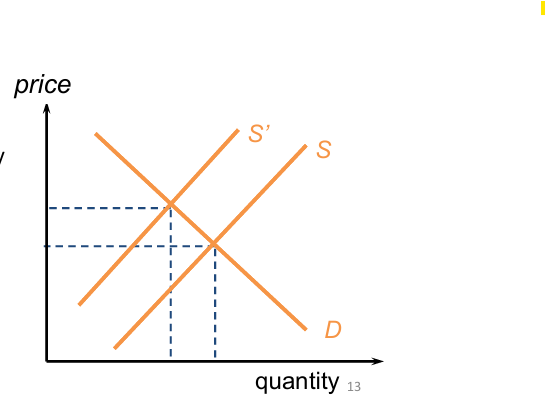
  • market labour supply curve

  • shifts caused by: # qualifications, NW benefits, cost of jobs (S’ —> S)

Responsiveness level to change in wages depends on:

• difficulty to change jobs

• LR or SR

Wages will rise more with demand if supply is more inelastic

Marginal Revenue Product of Labour (MRPL):

The change in TR revenue due to employing one more unit of labour

Marginal Cost of Labour (MCL):

MCL is the change in TC due to employing one more unit of labour

Relation between marginal input rule and marginal output rule:

(1) Marginal input rule: so long as the firm does not shut down, a buyer should employ the number of units of labour where

<aside> 💡

*marginal revenue product of labour) MRPL = MCL (marginal cost of labour)

</aside>

• MRPL: The change in TR due to +1 unit of labour

• MCL: The change in TC due to +1 unit of labour

• MRPL > MCL —> +1 unit —> TR increase > TC increase

(2) Relation to the Marginal output rule:

<aside> 💡

MRPL = MR x MPPL (MR x Marginal physical product of labour)

</aside>

MRPL = MPPL x MR = MC

MR = MCL / MPPL = cost of extra UoL / n. units it produces (extra cost of producing one of those units of output)

Therefore, Marginal input rule and Marginal output rule are effectively the same

Assumptions for perfectly competitive labour markets:

• A1 Buyers of labour (firms) operate in a perfectly competitive output market

  • Can sell as much as they want at current price without affecting price, p = MR

  • MRPL = MR x MPPL = p x MPPL

• A2 Buyers of labour are wage takers in the labour (input) market

  • Can employ as much as they want at current wage rate without affecting wage rate, MCL = w

• A3 Complete information

  • Workers are aware of available jobs and their conditions

  • Employers know quantity of available labour and productivity level

• A4 Workers are wage takers

  • Cannot influence market price

    • Can supply as much labour at a given wage

    • Choice —> NO reaction from other workers

• A5 Free entry for workers

  • No incurring costs, movement restrictions, no union barriers

  • Takes time and entry = LR

Characteristics of perfectly competitive labour markets:

• Many small sellers (workers)

• Low barriers to entry

• Undifferentiated seller substitutability

• Many small buyers (firms)

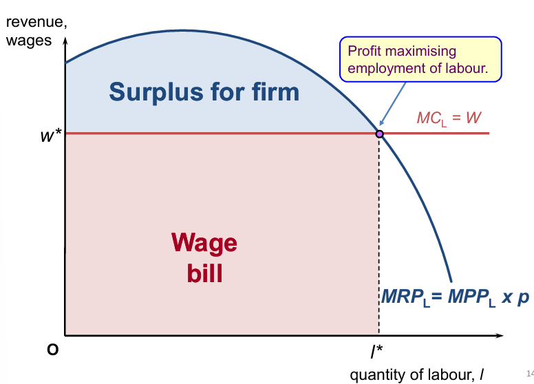
Pmax position for an individual firm in the labour market:

• same curve shape as MPPL curve

• Pmax = I* and W* intersected

• Surplus is where quantity is above wage bill; any quantity before I* > wage bill, so below Pmax

• if output price falls; MRPL1 shifts down to MRPL

  • I1 shifts left to I2,

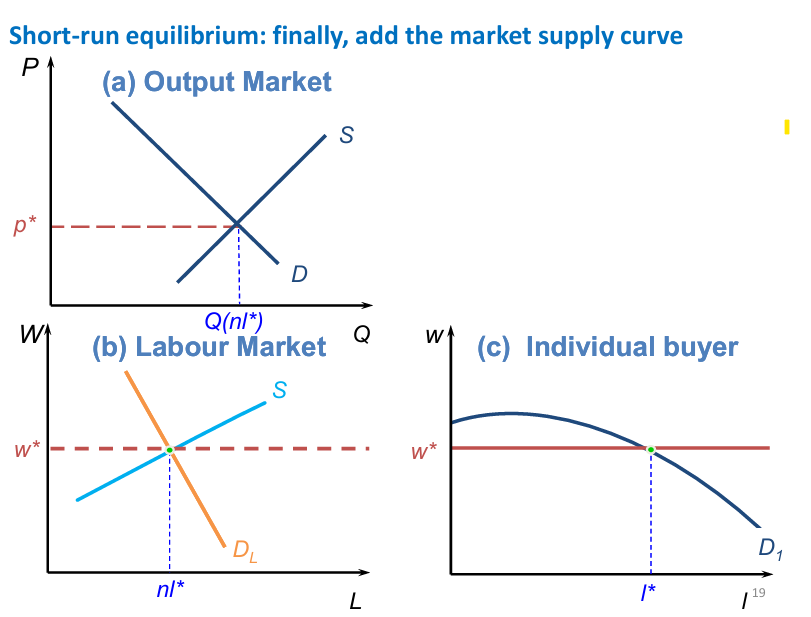
SR EQ in the Labour Market:

• Buyers choose optimal employment levels

• Sellers choose optimal supply levels

• Sellers supply as much as buyers want to purchase

Product market price is determined by S&D

Market wage is determined by market S&D

Seller’s output is determined seller-specific S&D

Monopsony assumptions:

Assumptions

• Perfectly competitive

• Complete information

• Workers = wage takers

• Free entry

A2 - the firm is a wage maker in the labour market; can influence the wage at which it employs labour

Monopsony market characteristics:

• undifferentiated workers

• complete information

• Workers are equally productive and buyers and sellers are fully informed

• Many small sellers (workers)

• One large buyer (firm)

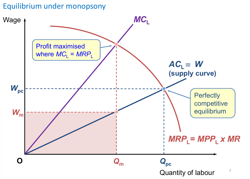
Equilibrium under Monopsony and diagrammatic analysis:

+1 unit:

• another unit is employed at wage w, TCL increase w

• all other units are employed at a slightly higher wage, so TCL increase by sL

  • L represents the units employer at the lower wage

  • S represents how much the wage has risen (Supply curve slope)

• Supply curve = s = W = ACL (as established)

• MCL = left of the SC as MCL > ACL

• MRPL = MPPL x MR (as established) - how much TR rises if +1 unit employed

• Pmax is where MCL = MRPL at Qm

  • Qm = how much labour the Monopsony should employ

  • Wm = wage rate at which the Monopsony should employ

Comparing Equilibrium under Monopsony and Perfect Competition:

• COMPARISON: Perfectly Competitive EQ is where Qpc = Wpc on ACL curve

  • Q is higher and W is higher at pc, but there is now only one firm and thus a wage maker and can employ more workers are lower wages.

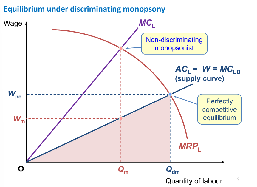
Discriminating Monopsony:

• there are Lpc units of labour employed

• This is determined by the intersection of MCLD and MRPL

• Same units of labour employed as under perfect labour markets but wage bill is lower, so the surplus for the firm is larger

• There is no deadweight loss

• at Qdm, wage rate is higher compared to non-discriminating

Monopoly Union Assumptions:

• Perfectly competitive output market

• Complete information

• Firms = wage takers

• Free entry

• Workers are wage makers; each worker is a member of a union, facing no outside competition

  • common interest of maximising insider wages and employment

  • Assume the union sets a minimum wage

Evaluation of Monopoly Union:

• Benefits those in employment

• Benefit’s their members by increasing wages

• Higher wages —> lower total employment

• Harms those who became unemployed and those who purchase output as price = higher

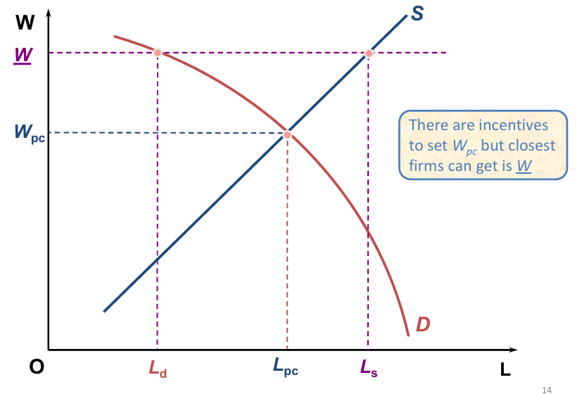
Monopoly Union and diagrammatic analysis:

• Increased wages —> higher TC and exit —> lower EMP and Higher prices

  • shift from S to S’ at lower Q and higher Price

• No union: wage determined by intersection between Wpc and Lpc

• With union: Minimum wage —> perfectly elastic supply curve at W

  • at W (above Wpc)< employment falls from Lpc to Ld

• Unemployment = Ls-Ld

  • Ls = units of labour want to be employed at MWR

  • Ld = units actually employed

• Benefits those in employment

• Harms those who became unemployed and those who purchase output as price = higher

Bilateral Monopoly assumptions

• perfectly competitive output market

• Complete information

• Free entry

• Firm = wage maker

• Workers = wage maker

  • both can influence wages

Bilateral Monopoly characteristics:

• undifferentiated workers

• complete information

• One large worker (union)

• One large buyer (large change)

Efficiency and equity in markets:

Efficiency:

• in what ways are the allocation of resources socially desirable

  • efficiency and equity

    • efficiency: size of the pie, big as possible

    • Equity: how the pie is divided

• when will the allocation of resources be socially desirable and when not?

• if not socially desirable, what is the best policy to resolve the problem?

Productive efficiency:

Allocation of resources within a firm; production at lowest possible cost

Allocation of resources among firms; TQ at lowest cost

MC = MR

Allocative efficiency:

Optimally distributing resources to maximise consumer satisfaction

No gain should be made by reallocation; gains are maximised

P = MC

Type of firms and if they are allocative or productively efficient (list them):

Type of Firm	Allocative Efficiency (P = MC)?	Productive Efficiency (Min AC = MC)?
Monopoly	✅ Yes (in the long run)	✅ Yes (in the long run)
Perfect Competition	❌ No	❌ No
Monopolistic Competition	❌ No	❌ No
Oligopoly	❌ No	❌ No (unless behaving like perfect competition)
Natural Monopoly	❌ No	✅ Yes (can exploit economies of scale)
Monopsony	❌ No (restricts input purchases)	❌ No (may not operate at minimum AC)

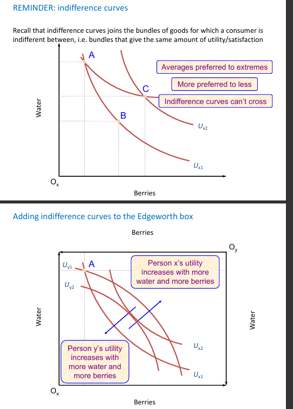
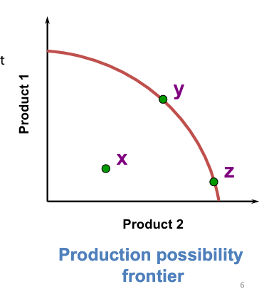
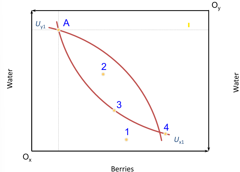
How can indifference curves being added to the Edgeworth box create Pareto improvements and optimal resource allocation (explain diagrams)

• Bundle C > Bundle B as more is preferred to less

• Bundle B > Bundle C are more is preferred to less and average is preferred to extremes

• Person X utility increases with more water and berries as it requires more of both good, and more is preferred to less / average > extreme

  • Person X moves closer to origin Oy as it increases volume

• Person Y utility increases with more water and berries as it requires more of both good, and more is preferred to less / average > extreme

  • Person Y moves closer to origin Ox as it increases volume

• This brings X and Y closer to the Pareto optimal point

• Pareto improvement is present as Person Y and X are better off without harming the other person ‘s utility

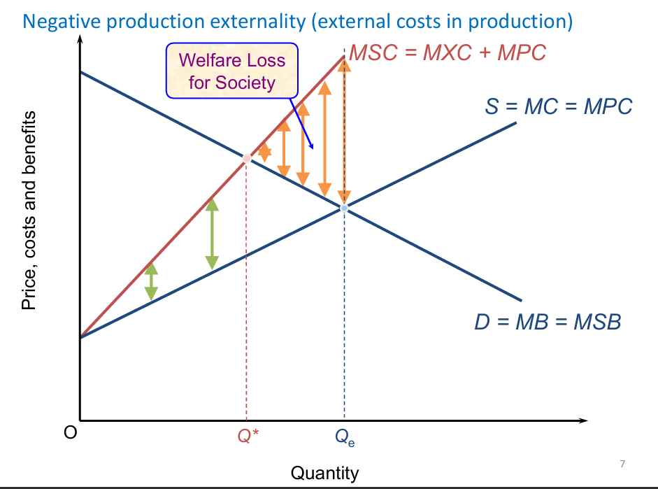
Pareto improvements:

• Bundle 1 - Person X is better off as their utility increases as they move closer to their indifference curve Ux1 but Person Y is worse off as they exceed their optimal indifference curve Uy1 ☹

• Bundle 2 - utility of Person X and Y both increases without crossing the alternative indifference curve, thus neither are worse off 🙂

• Bundle 3 - utility of Person X and Y both increases without crossing the alternative indifference curve, thus neither are worse off (person Y reaches X indifference curve but does not cross it) 🙂

• Bundle 4 - Person Y is worse off as this bundle lies to the right of their indifference curve ☹

Characteristics and types of externality:

• Positive: External benefit to a third party

  • not enough produced in a market

  • positive production e.g. new airports and technological research

  • positive consumption e.g. education and immunisations

• Negative: External cost on a third party

  • too much produced in a market

  • negative production e.g. air and water pollution

  • negative consumption e.g. loud music and cigarette smoking

• Production and consumption externality

• Banning all products with negative externalities is not socially desirable e.g. ban all cigarettes

  • amount with best trade off is recommended

Negative production externality diagram:

• Qe is where marginal social benefit = marginal benefit and marginal private cost = marginal cost (demand and supply) meet

  • Demand = benefit as consumers benefit from output

  • supply = cost as firms have to pay for production and is thus a cost

• There is a welfare loss for society above the demand curve and is greater at higher quantities above Q*

• Q* is the optimal equilibrium where quantity is lower and prices, C&B are higher; this means less external costs of production, bringing society closer to the socially optimum equilibrium

  • Welfare loss decreases as you move closer to the SOE

  • Negative production externalities cannot be zero as it is not optimal, but should be at a lower desired Q

• Therefore, Qe —> Q*, quantity falls and price increases, so NEX decreases

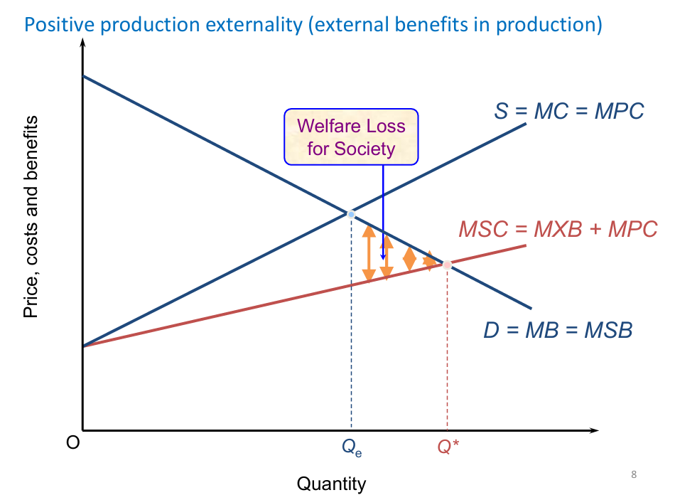
Positive production externality diagram:

• Qe is where marginal social benefit = marginal benefit and marginal private cost = marginal cost (demand and supply) meet

  • Demand = benefit as consumers benefit from output

  • supply = cost as firms have to pay for production and is thus a cost

• There is a welfare loss for society below the demand curve and is greater at lower quantities above Q*

• Q* is the optimal equilibrium where quantity is higher and price are lower; this means more external benefits in production, bringing society closer to the socially optimum equilibrium

  • Welfare loss decreases as you move closer to the SOE

  • Positive production externalities cannot be very high as it is not optimal, but should be at a lower desired Q

• Therefore, Qe —> Q*, quantity rises and price decreases, so PEX increases

Pigovian taxes and pollution:

e.g. pollution

• Government can either

  • regulation: restrict waste to Y units of pollution per unit of output

  • Pigovian tax: each firm pays T per unit of output

    • reduces pollution, more efficient at pollution reduction, environmentally friendly, raises money for government

Social efficiency in terms of externalities:

• social planners would intervene in socially inefficient markets

• market based policies can be used e.g. per unit taxes and per unit subsidies

  • tax if production is too high (Pigovian tax)

  • subsidise if production is too low

    • thus internalising the externality and aligning private incentives with social efficiency

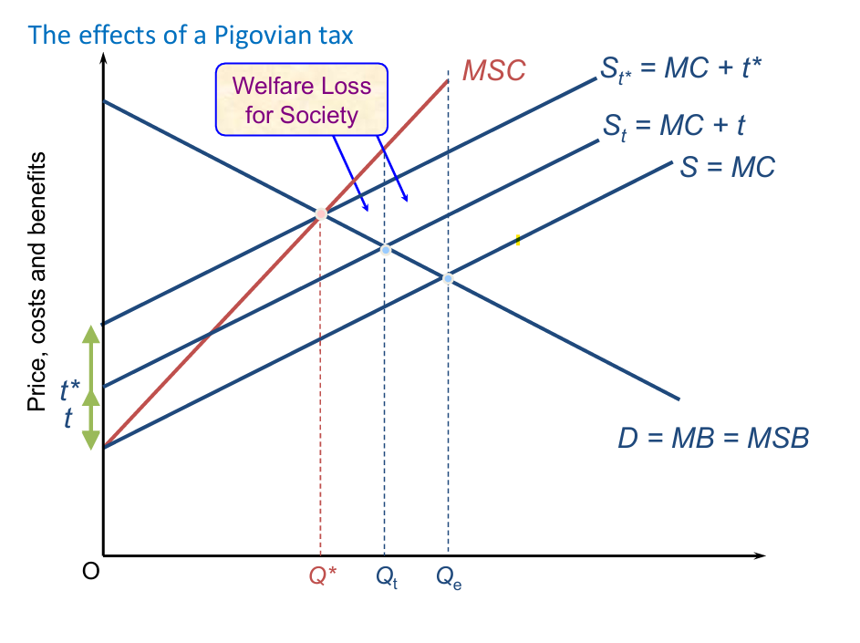
Effects of a Pigovian tax in a diagram:

• Pigovian taxes increases prices from t to t* and restrict output from Qe to Qt

  • t* is a certain level of Pigovian tax but not the optimal (t), while output still does fall

  • Both are closer to Q* SOE

    • St* = MC + t* at Q* (which is the optimal tax level, any further taxes may cause tax evasion or market exit)

  • Welfare loss for society decreases as production of negative externalities falls and government tax revenue increase

Rival product and its types:

• Rival Product: A product where one person's consumption reduces availability for others (e.g., food, clothing).

  • some can be consumed by only one person

  • some can be consumed by multiple but not simultaneous

  • some can be consumed by multiple but not by another person at the same time

Non-rival product:

Non-Rival Product: A product that multiple people can consume without reducing its availability (e.g., public parks, digital content).

Excludable products and its types:

Excludable: consumers can be excluded from the benefits of a product

• products from which non-payers could be and are excluded e.g. private gym memberships

• products from which non-payers could be and are NOT excluded

Non-excludable products:

consumers can be excluded from the benefits of a product .g. streetlights / national defence

Table of (non) rival and (non) excludable goods (give 2 examples of each combo):

	Rival	Non-rival
Excludable	textbooks / loaf of bread / cinema tickets / congested motorways (Private goods)	tv channels / motorways like tolls or uncongested (club goods)
Non-excludable	fish in the ocean (common resources)	Streetlights / firework displays / small roads (public goods)

Theory and solution of Free-Rider problem:

• The product is underproduced even though societal value > cost of providing it

• e.g. fireworks display, which is under-provided

  • supplier choose to ignore external benefit (such as non0-buyers being provided external benefits)

• Solution: gov pays for the display and recoups costs through taxation

Definition of Free-Rider:

Free Rider: a person who receives the benefit of a good but does not pay for it

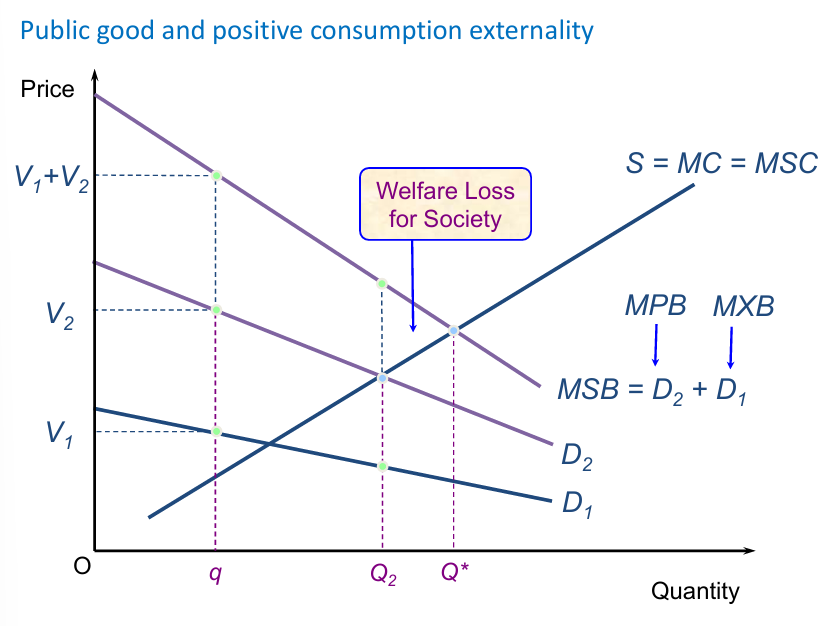
Free-rider problem as a diagram (explain):

• q = quantity of fireworks

• V1 = MPB for person 1 on their demand curve ; free-rider, so demand is lower at MXB (did not pay)

  • person 1 buys so Q is higher where Q2 meets D2 (compared to D1 Q1 for free rider)

• V2 = MPB for person 2 on their demand curve ; assumed as MPB, greater benefit than D1

• MSB = D2 + D1 (total private benefit)

• Supply curve = MC and MSC (no externalities in production

• Q* = optimal SOE

• Welfare loss = diff between MSB and MSC for the units not provided, market provides level of Q2

Solution to the Tragedy of the Commons:

• Solution: property rights and rules

  • Farmers who own land with legally protected property rights have an incentive to invest in better irrigation, fertilizers, and sustainable practices. Without secure property rights, they may fear land seizure and avoid long-term investments, leading to lower productivity and inefficient land use.

    • This allows farmers to protect and improve their own land, preventing env. degradation in which government / private bodies will regulate farmer activity

    • Promotes sustainability, sustains profits for farmers and reduces env. degradation

    • However, due to scale and private incentives, implementation and regulation is difficult

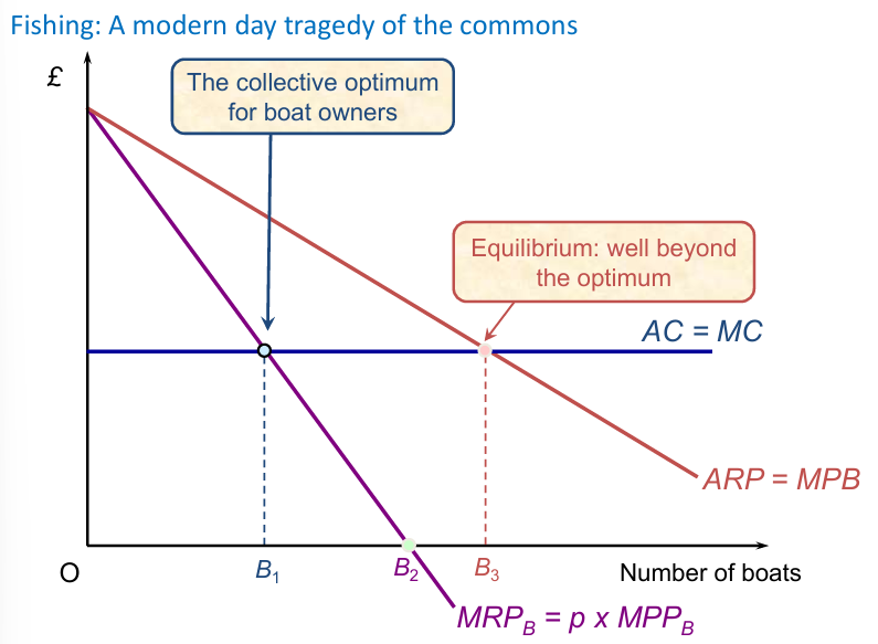
Explanation of the diagram for the Tragedy of the Commons (fishing)

• AC = MC = MPC

• ARP = AR per boat —> MPB

  • Equilibrium is beyond optimum at higher Q to increase revenue (B3)

  • This is where tragedy of the commons occur as B3 > B2

• B1 is collective optimum to prevent significant env. degradation (SOE)

  • this is where MSB = MSC where B1 meets D curve

• Solution: property rights and rules

Imperfect information:

Imperfect information:

• Buyer lacks information about prices

• Buyer’s behaviour determines level of information

• Firms have market power

Asymmetric information:

• One side lacks more information than the other side

• Lack of information determines behaviour

• High quality markets may not exist

Theory example of Imperfect information:

• two firms sell an identical product; costs = c, consumers want to buy one unit, consumers value products at v < c, consumers know both prices and are willing to shop at either

• Perfect : When Consumers have perfect info, they receive all benefits from trade

• Imperfect: Consumers do not know the prices and finding info is costly

  • When Consumers are uniformed about prices and finding info is costly, they receive no trade benefits

The Unravelling Principle

The Unravelling Principle

• Firms have incentives to provide info for the uniformed

Holds if:

• Product differentiation is important to consumers

• Costless, credible statements about products can be made by firms

Intuition —> no info —> all firms ‘average’; random selection

• Firm offering best terms > average —> should disclose info to increase consumers

3 types of goods under Asymmetric information:

• Search goods: easy to assess quality pre-purchase 🙂

• Experience goods: difficult to assess quality pre-purchase :]

• Credence goods: difficult to assess quality pre and post purchase 😟

The Problem of Adverse Selection

To buy the cars, it costs the firm : £3000 for a high quality car / £100 for a low quality car

Consumers are willing to pay: £4000 for a high quality car / £1000 for a low quality car

Firms could make: £1000 from selling a high quality car / £900 from selling a low quality car

• consumers cannot tell the diff in quality (experience goods)

• Average willingness to pay = (4000+1000) / 2 = 2500

• Uninformed consumer choosing at random is willing to pay £2500

Salesperson would make a loss of £500 if they sell high quality car at what consumers are willing to pay —> only low-quality cars will be bought and sold

• market for high quality cars affected —> adverse selection affected by asymmetric information

3 Solutions to Informational Problems in a market:

Types	Example
Signalling	high quality claim credible such as fixing cars for free if they break down
Screening	buyers get information on firm’s reputation e.g. reviews, TripAdvisor
Government intervention	minimum standards, verifying firm’s claims, providing information or publicising it